4 Farm typologies
This chapters proposes a step-by-step method to understand farm diversity and select representative farms for e.g., on-farm experiments.
4.1 Concept of farm typology
Farm typologies aims at characterizing the diversity of farming systems and their distribution in heterogenous communities, as a basis for prioritizing interventions (Hammond et al. 2020) and/or to select representative farms, or ‘prototype farms’ (Alvarez et al. 2018).
Various methodologies, all with their strengths and their weaknesses, are commonly used to delineate typologies, from (quantitative) statistical typology (Tittonell et al. 2010) to (qualitative) expert-based typology involving farmers and other knowledgeable stakeholders (Kebede 2009).
Here, we are using a method of statistical typology delineation developed by Hassall et al. (2023). One of the key strength of the method is that non-metric multidimensional scaling can be used, allowing for the selection of qualitative variables, not only quantitative ones, for typology delineation.
In the example below, we will use the small dataset we created in the previous chapter (and that was saved as a rds file). You can also download it here (and load it with the function read.csv()): https://github.com/FBaudron/Supporting-codesign/blob/main/04-typologies/small_dataset.csv
A standalone R script containing the full workflow is available at the following link: https://github.com/FBaudron/Supporting-codesign/blob/main/04-typologies/typology.R.
4.2 Data preparation
We begin by clearing the environment, ensuring all necessary packages are installed and loaded, and importing the data.
rm(list = ls())


if (!require("openxlsx")) install.packages("openxlsx")
if (!require("vegan")) install.packages("vegan")
if (!require("ade4")) install.packages("ade4")
if (!require("dendextend")) install.packages("dendextend")
if (!require("gtsummary")) install.packages("gtsummary")
if (!require("kableExtra")) install.packages("kableExtra")
if (!require("splitstackshape")) install.packages("splitstackshape")
if (!require("NbClust")) install.packages("NbClust")
if (!require("randomForest")) install.packages("randomForest")


library(openxlsx)
library(vegan)
library(ade4)
library(dendextend)
library(gtsummary)
library(kableExtra)
library(splitstackshape)
library(NbClust)
library(randomForest)

data = readRDS("small_dataset.rds")
# data = read.xlsx('small_dataset.xlsx', sheet = 1)
We first rename some variables, recode some categorical variables into binary ones, and convert NAs into zeros for some variables.
names(data)[c(1, 4:6, 27, 29, 33:36)] = c("ID", "age_hhh", "sex_hhh", "edu_hhh",
    "cover_crops", "integrated_pest_management", "homemade_feeds", "fodder_production",
    "fodder_preservation", "survival_feeding")

data$sex_hhh = as.numeric(data$sex_hhh == "Female")

data$edu_hhh = as.numeric(data$edu_hhh != "Primary level")

data$main_food_source = as.numeric(data$main_food_source == "Own production")

data$main_income_source = as.numeric(data$main_income_source == "Crop sales" | data$main_income_source ==
    "Livestock sales")

data[c(23:36)][is.na(data[c(23:36)])] = 0
4.2.1 Removing outliers
We remove extreme values to avoid skewing the analysis. For this, we plot and examine boxplots. Points beyond the whiskers of the boxplot have values higher than 1.5 times the interquartile range and are considered potential outliers. When such extreme points are observable, we remove them from the dataset.
Age of the head of the household doesn’t have any true marked outlier.
boxplot(data$age_hhh)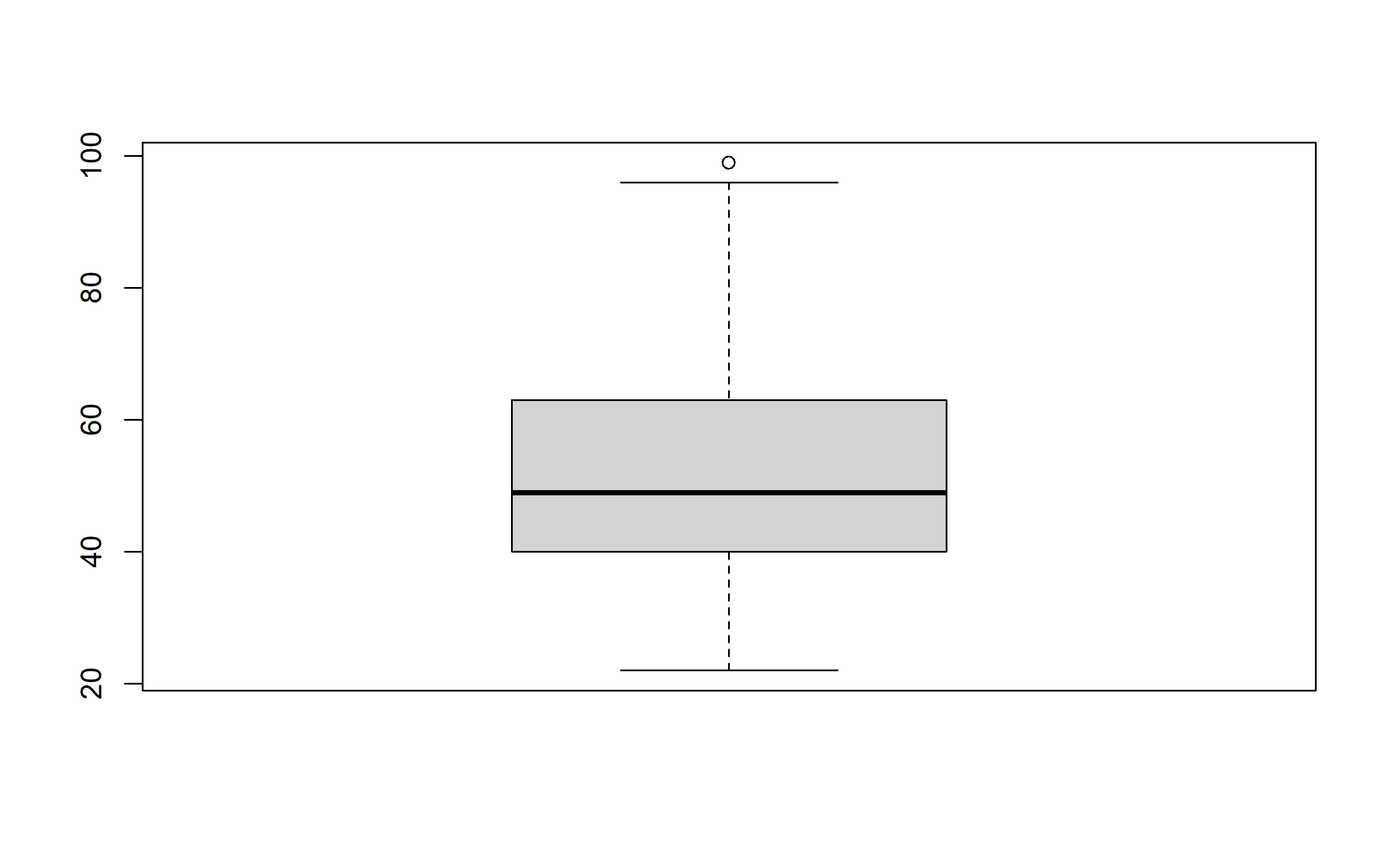
But family size does.
boxplot(data$family_size)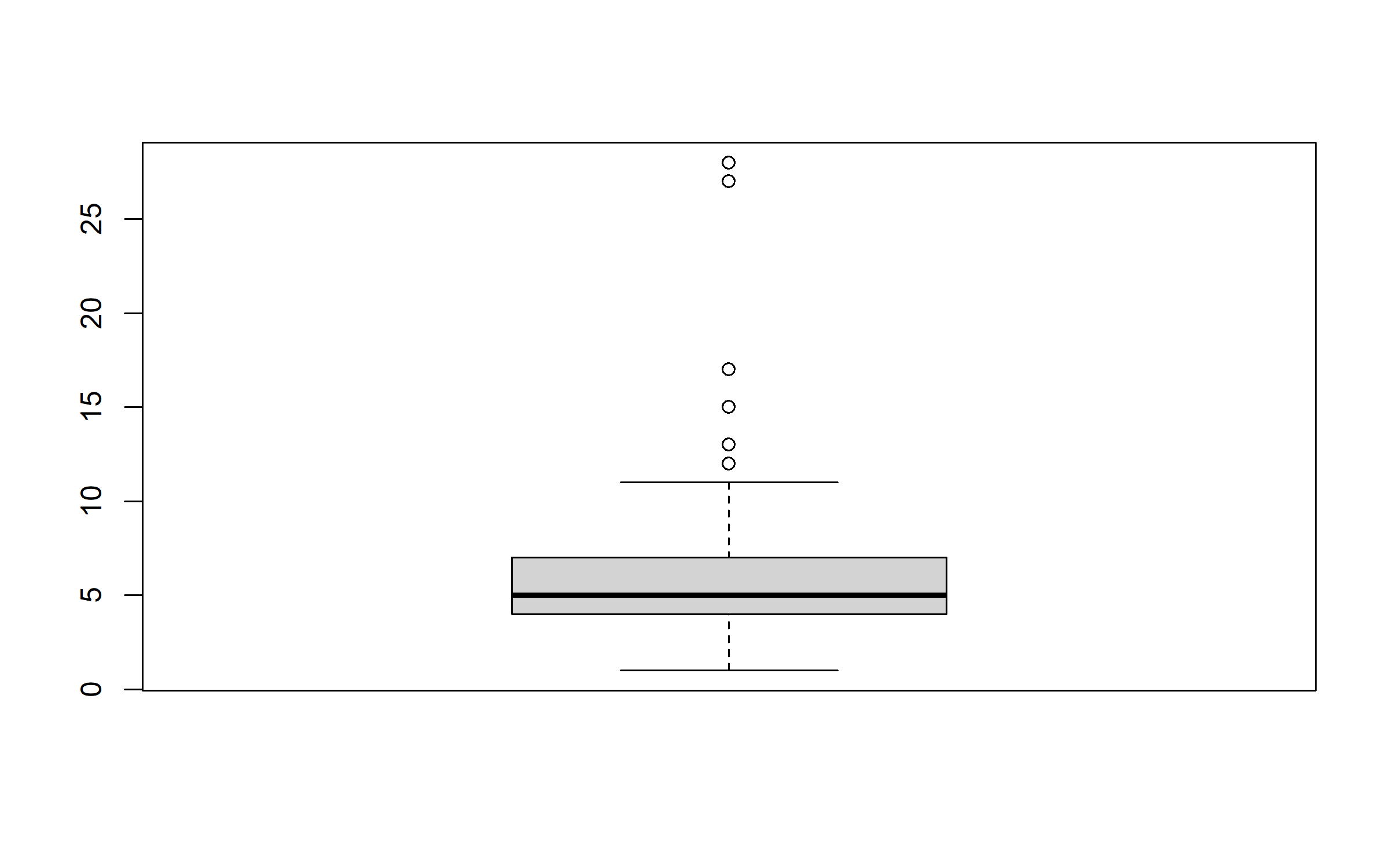
Thus, we remove all records with a family size greater than 20.
data = data[data$family_size < 20, ]
boxplot(data$family_size)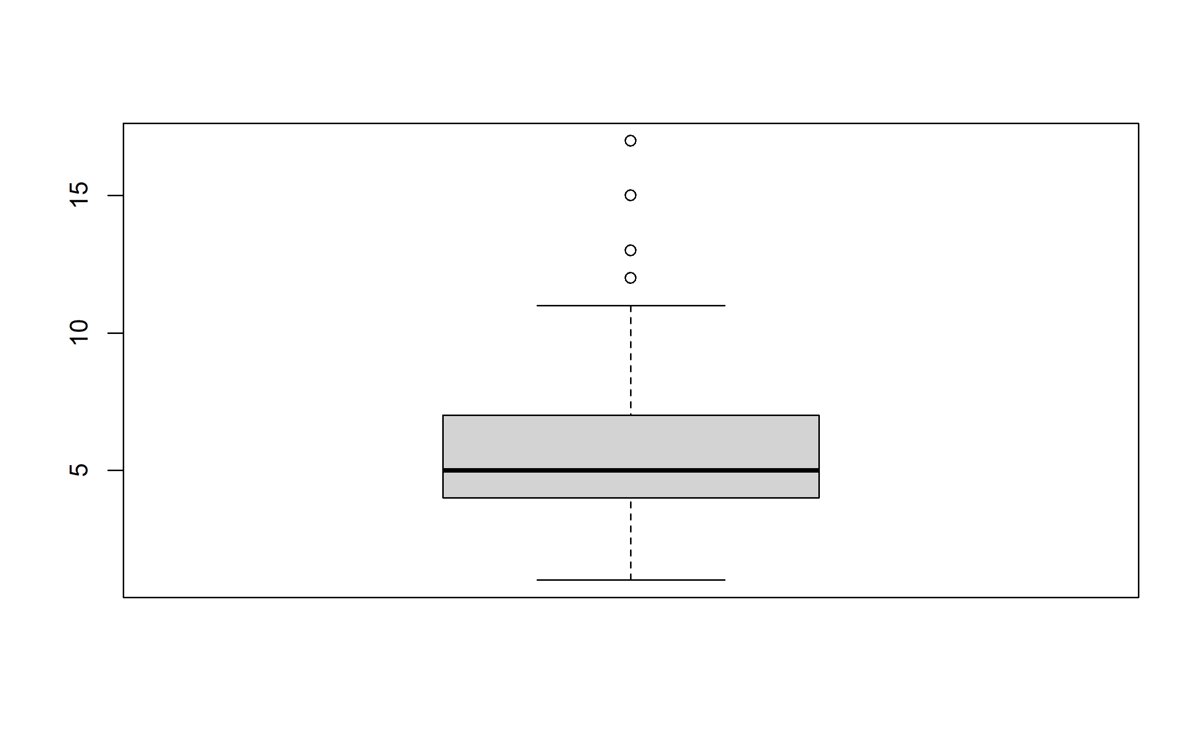
We inspect all other continuous variables, and find outliers for the number of small ruminants, the number of poultry, livestock offtake, and equipment value. We remove these extreme values from the dataset that we will use to delineate the farm typology.
# boxplot(data$cropped_area)

# boxplot(data$fallow)

# boxplot(data$prop_non_cereals)

# boxplot(data$fertilizers)

# boxplot(data$amendment)

# boxplot(data$cattle)

# boxplot(data$small_rum)
data = data[data$small_rum < 100, ]
# boxplot(data$small_rum)

# boxplot(data$poultry)
data = data[data$poultry < 400, ]
# boxplot(data$poultry)

# boxplot(data$food_security)

# boxplot(data$hdds)

# boxplot(data$tot_div)

# boxplot(data$cereal_prod)

# boxplot(data$offtake)
data = data[data$offtake < 6, ]
# boxplot(data$offtake)

# boxplot(data$eq_value)
data = data[data$eq_value < 8000, ]
# boxplot(data$eq_value)
4.2.2 Normalization of continuous variables
To reduce the influence of extreme values, continuous variables are log-transformed.
We create first a copy of the dataset before data transformation.
typo = dataWe plot histograms of continuous variables, and when distribution departs too much from a Gaussian distribution, we logtransform the variable. In that case, we take care of adding a term - half of the minimum positive value - to avoid passing zeros to log10.
Age of the head of the household has a relatively Gaussian distribution.
hist(typo$age_hhh)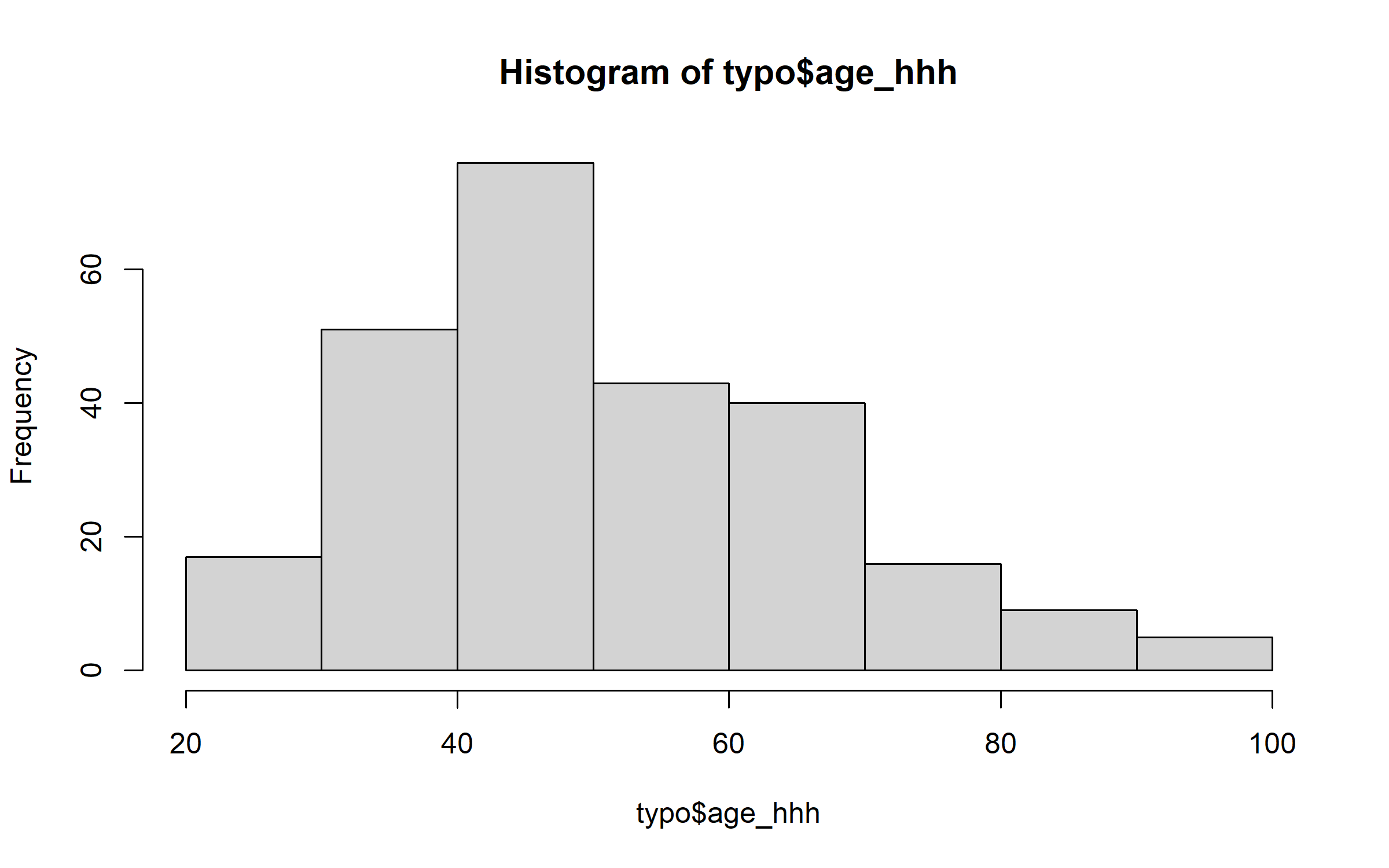
But family size has a distribution that departs markedly from a Gaussian distribution.
hist(typo$family_size)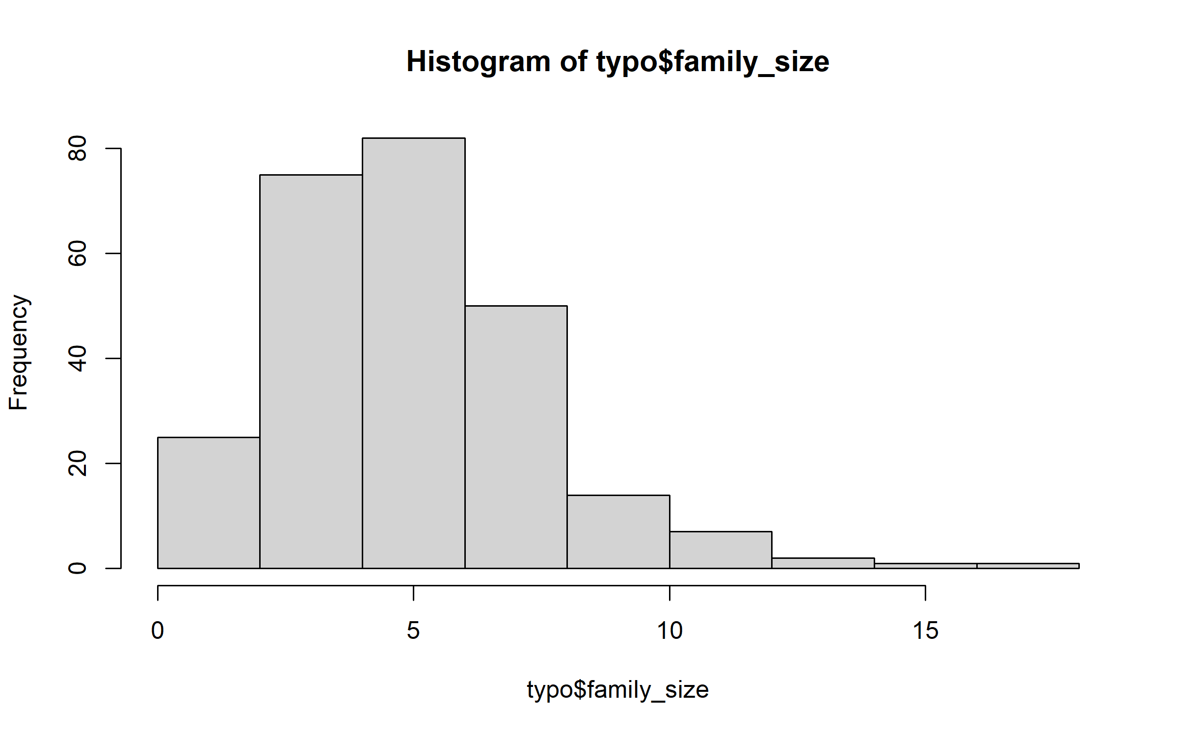
Thus, we logtransform the variable family size.
typo$family_size = log10(typo$family_size + (0.5 * min(typo$family_size[typo$family_size >
    0], na.rm = TRUE)))
hist(typo$family_size)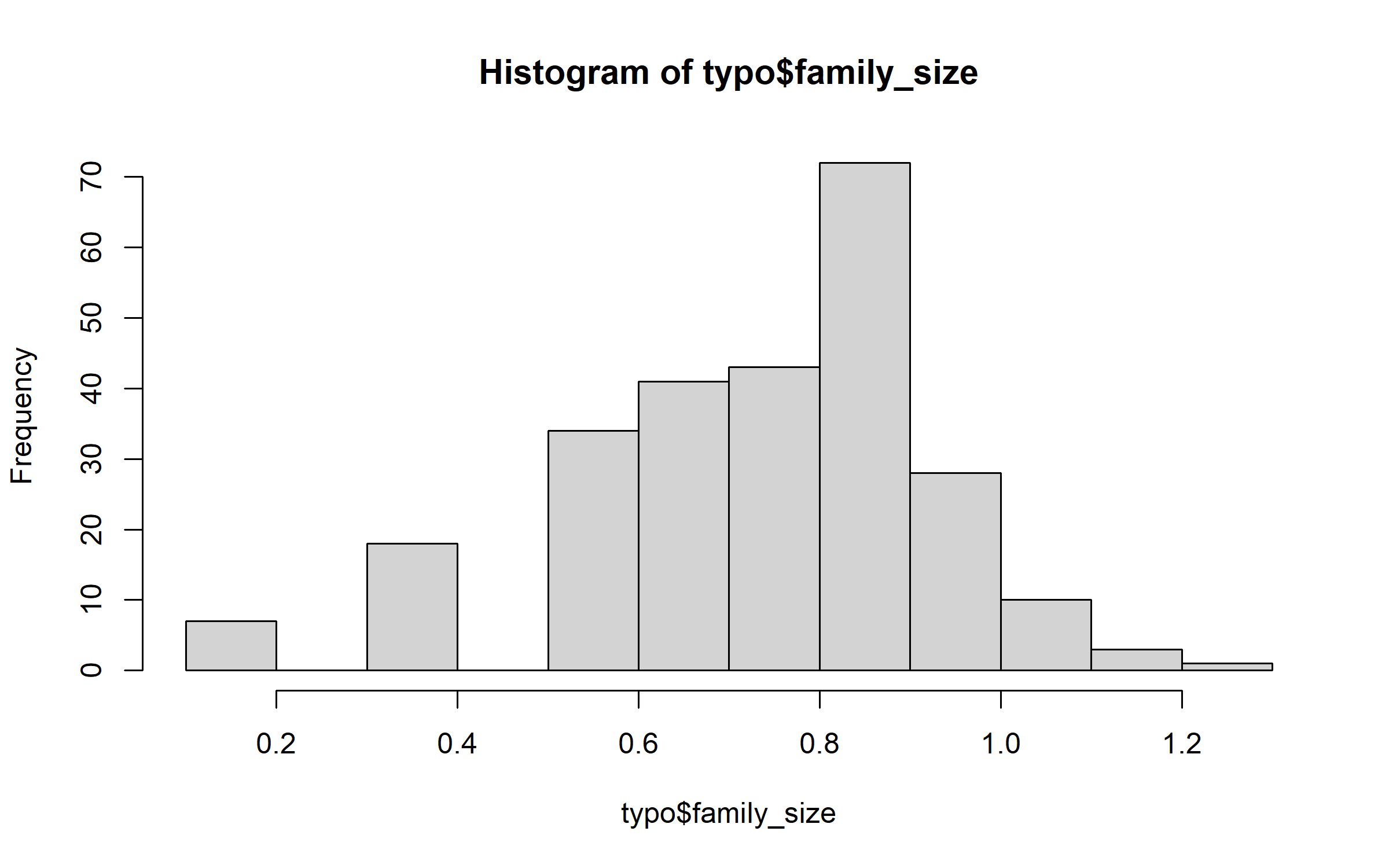
We inspect all other continuous variables, and find the total cropped area, the fallow area, the total quantity of fertilizer used, the total quantity of organic amendments used, the number of cattle, the number of small ruminants, the number of poulty, the total quantity of cereal produced, the livestock offtake, and the equipment value to depart markedly from a Gaussian distribution. We therefore log-transformed these variables.
# hist(typo$cropped_area)
typo$cropped_area = log10(typo$cropped_area + (0.5 * min(typo$cropped_area[typo$cropped_area >
    0], na.rm = TRUE)))
# hist(typo$cropped_area)

# hist(typo$fallow)
typo$fallow = log10(typo$fallow + (0.5 * min(typo$fallow[typo$fallow > 0], na.rm = TRUE)))
# hist(typo$fallow)

# hist(typo$prop_non_cereals)

# hist(typo$fertilizers)
typo$fertilizers = log10(typo$fertilizers + (0.5 * min(typo$fertilizers[typo$fertilizers >
    0], na.rm = TRUE)))
# hist(typo$fertilizers)

# hist(typo$amendment)
typo$amendment = log10(typo$amendment + (0.5 * min(typo$amendment[typo$amendment >
    0], na.rm = TRUE)))
# hist(typo$amendment)

# hist(typo$cattle)
typo$cattle = log10(typo$cattle + (0.5 * min(typo$cattle[typo$cattle > 0], na.rm = TRUE)))
# hist(typo$cattle)

# hist(typo$small_rum)
typo$small_rum = log10(typo$small_rum + (0.5 * min(typo$small_rum[typo$small_rum >
    0], na.rm = TRUE)))
# hist(typo$small_rum)

# hist(typo$poultry)
typo$poultry = log10(typo$poultry + (0.5 * min(typo$poultry[typo$poultry > 0], na.rm = TRUE)))
# hist(typo$poultry)

# hist(typo$food_security)

# hist(typo$hdds)

# hist(typo$tot_div)

# hist(typo$cereal_prod)
typo$cereal_prod = log10(typo$cereal_prod + (0.5 * min(typo$cereal_prod[typo$cereal_prod >
    0], na.rm = TRUE)))
# hist(typo$cereal_prod)

# hist(typo$offtake)
typo$offtake = log10(typo$offtake + (0.5 * min(typo$offtake[typo$offtake > 0], na.rm = TRUE)))
# hist(typo$offtake)

# hist(typo$eq_value)
typo$eq_value = log10(typo$eq_value + (0.5 * min(typo$eq_value[typo$eq_value > 0],
    na.rm = TRUE)))
# hist(typo$eq_value)
4.3 Delineation of farm types
Next, we calculate dissimilariries and distances, reduce the dimensionality of the dataset through principal coordinate analysis, and delineate farm types through hierarchical cluster analysis.
We first remove records with missing values.
typo = na.omit(typo)4.3.1 Calculation of dissimilarities and distances
We calculate dissimilarities for 3 groups of variables: structural variables, functional variables, and adoption variables. Structural and functional variables are further divided into continuous and binary variables, for which different methods are used in the calculation of dissimilarities.
We first calculate the scaled euclidean dissimilarity between continuous structural variables using the function vegdist() of the R package vegan (Oksanen et al. 2025).
dEucs = vegdist(typo[, c("age_hhh", "family_size", "cropped_area", "fallow", "prop_non_cereals",
    "cattle", "small_rum", "poultry", "eq_value")], method = "gower")
Similarly, we calculate the scaled euclidean dissimilarity between continuous functional variables.
dEucf = vegdist(typo[, c("fertilizers", "amendment", "food_security", "hdds", "tot_div",
    "cereal_prod", "offtake")], method = "gower")
We then calculate the dissimilarity between binary structural variables using the function dist.binary() of the R package ade4 (Thioulouse et al. 2018).
dBin_ppls = dist.binary(typo[, c("sex_hhh", "edu_hhh", "bee_hives", "ind_garden",
    "com_garden")], method = 2)
Similarly, we calculate the dissimilarity between binary functional variables.
dBin_pplf = dist.binary(typo[, c("main_food_source", "main_income_source")], method = 2)Finally, we calculate the dissimilarity between binary adoption variables.
d_practices = dist.binary(typo[, c("community_seed_banks", "small_grains", "crop_rotation",
    "intercropping", "cover_crops", "mulching", "integrated_pest_management", "compost_manure",
    "tree_planting_on_farm", "tree_retention_natural_regeneration_on_farm", "homemade_feeds",
    "fodder_production", "fodder_preservation", "survival_feeding")], method = 2)
We combine the 2 dissimilarities of structural variables, weighing them by the number of variables in each dissimilarity.
We do the same for the 2 dissimilarities of functional variables.
d_structural = (9 * dEucs^2 + 5 * dBin_ppls^2)/14

d_functional = (7 * dEucf^2 + 2 * dBin_pplf^2)/9
We combine the three dissimilarity matrices — structural, functional, and adoption variables — into a single overall dissimilarity. Because the adoption component includes many binary variables, we downweight its contribution to avoid letting it dominate the resulting typology. Specifically, we multiply the adoption dissimilarity by 0.5 before combining, and then normalize by dividing by the sum of the weights (2.5) to keep the overall scale consistent. The factor of 0.5 used is arbitrary, but could be fine-tuned through iterations.
dAll = (d_structural + d_functional + 0.5 * d_practices^2)/2.5Finaly, we transform the matrix of dissimilarities to a matrix of distances.
distAll = sqrt(2 * dAll)4.3.2 Principal coordinate analysis & hierarchical cluster analysis
We reduce dimensionality while preserving distances using using principal coordinate analysis (PCO) implemented via the base R function cmdscale().
We select k axes to explain at least 50% of the variability .
pco = cmdscale(distAll, eig = TRUE, k = 10)
barplot(pco$eig[1:20])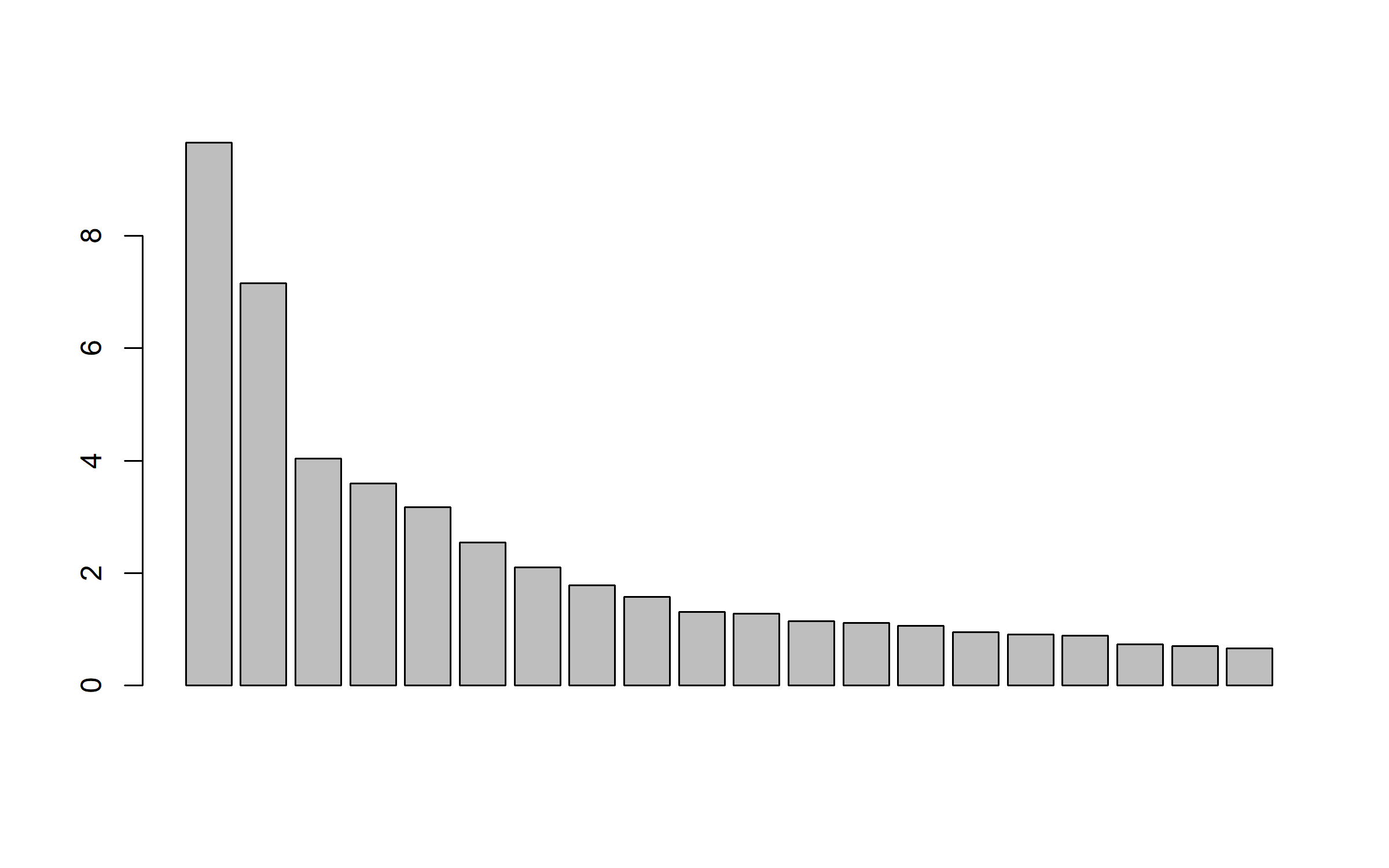
cum_var = cumsum(pco$eig)/sum(pco$eig)
k_axes = which(cum_var >= 0.5)[1]
k_axes
[1] 4We cluster farms based on PCO axes through hierarchical cluster analysis (HCA) carried out using the base R function hclust().
We plot the dendrogram.
pco_var = pco$points[, 1:k_axes]

hc_pco = hclust(dist(pco_var), method = "complete")
plot(hc_pco, hang = -1)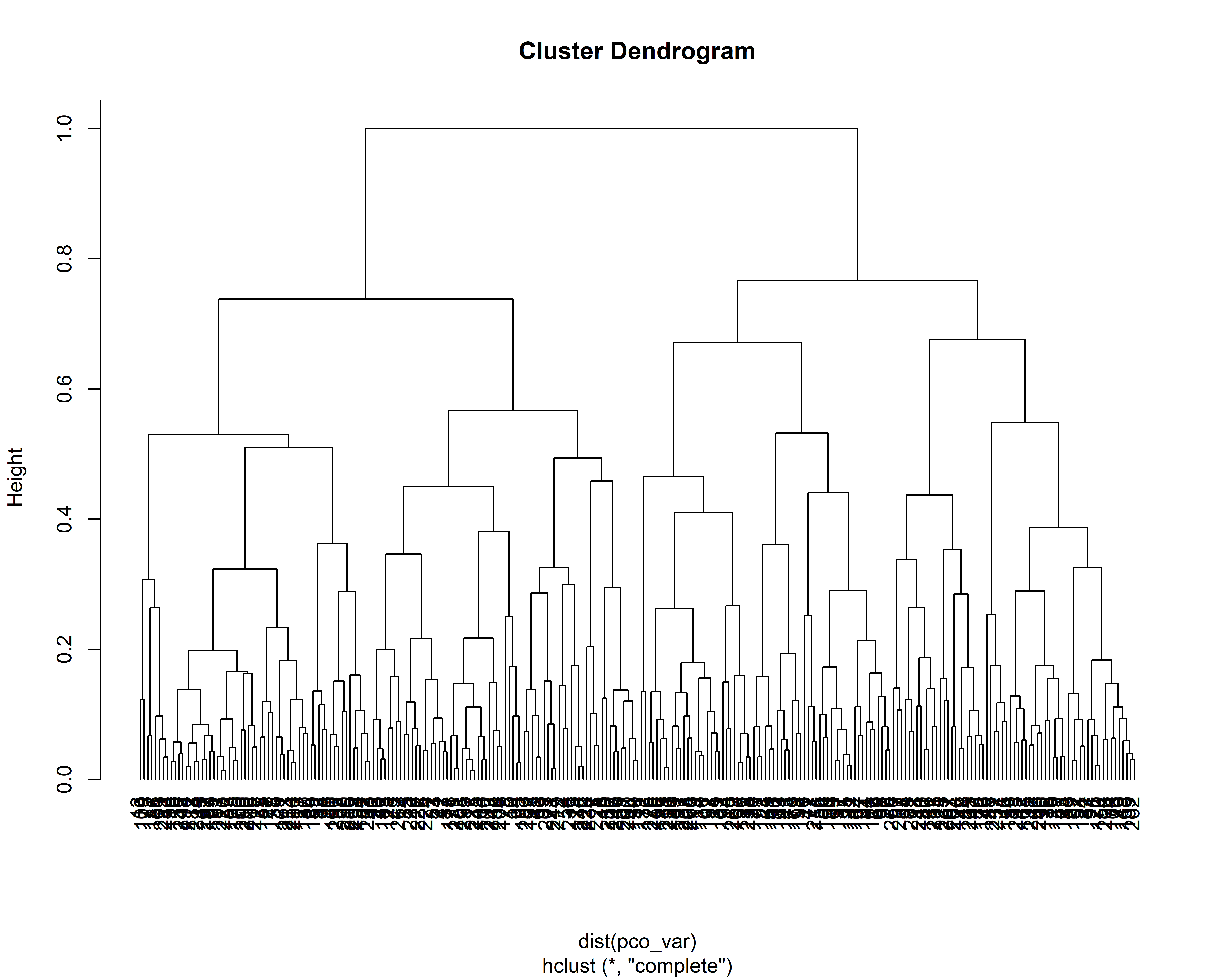
4.3.3 Selection of the number of clusters
We select the optimum number of clusters using the function NbClust() of the R package NbClust (Charrad et al. 2014), which computes multiple cluster validity indices (30 in our case) and compares them. The final number of clusters is determined using a majority rule, where each index ‘votes’ for a number of clusters and the number supported by the largest number of indices is chosen.
NbClust(pco_var, diss = dist(pco_var), distance = NULL, method = "complete")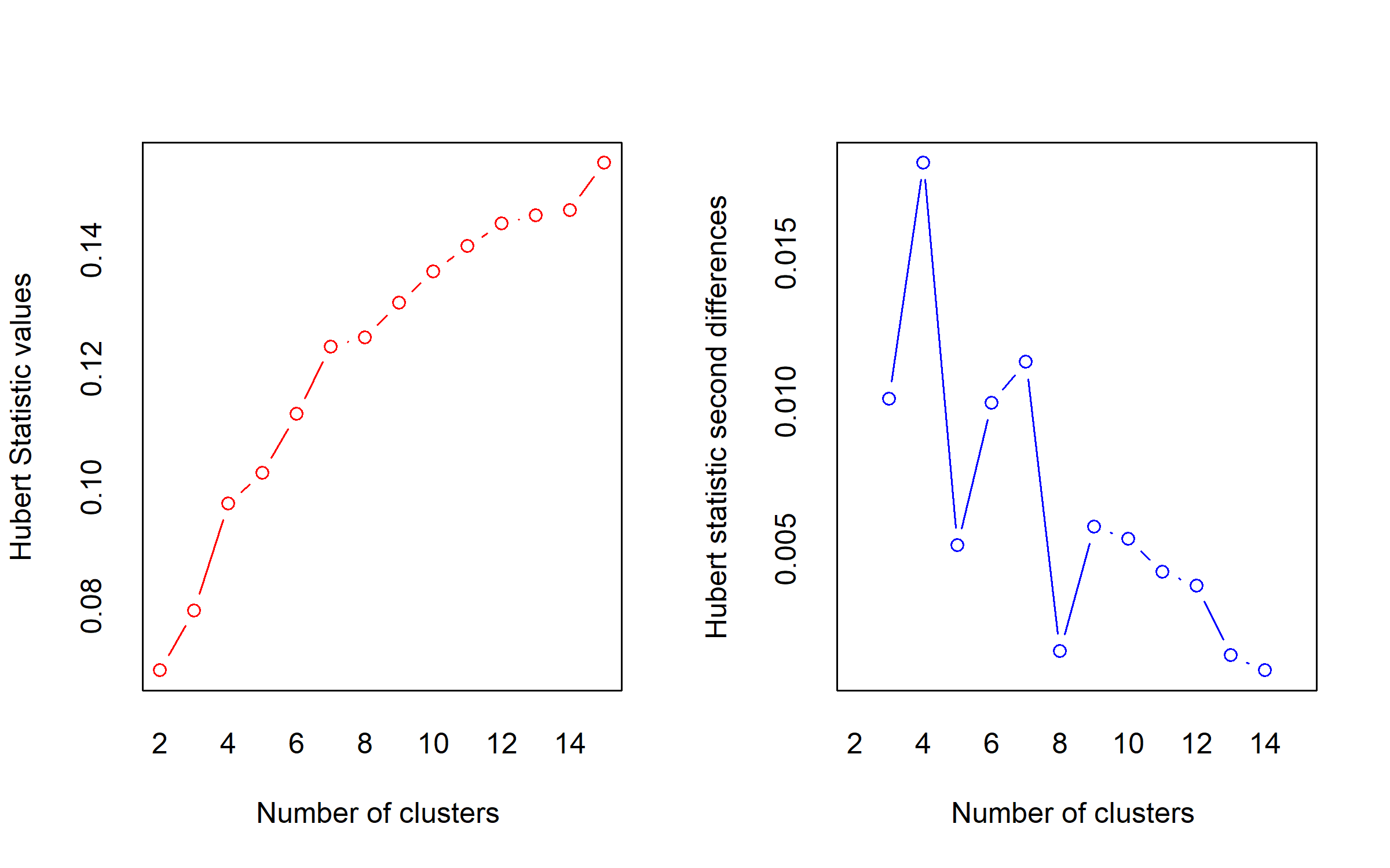
*** : The Hubert index is a graphical method of determining the number of clusters.
                In the plot of Hubert index, we seek a significant knee that corresponds to a
                significant increase of the value of the measure i.e the significant peak in Hubert
                index second differences plot.
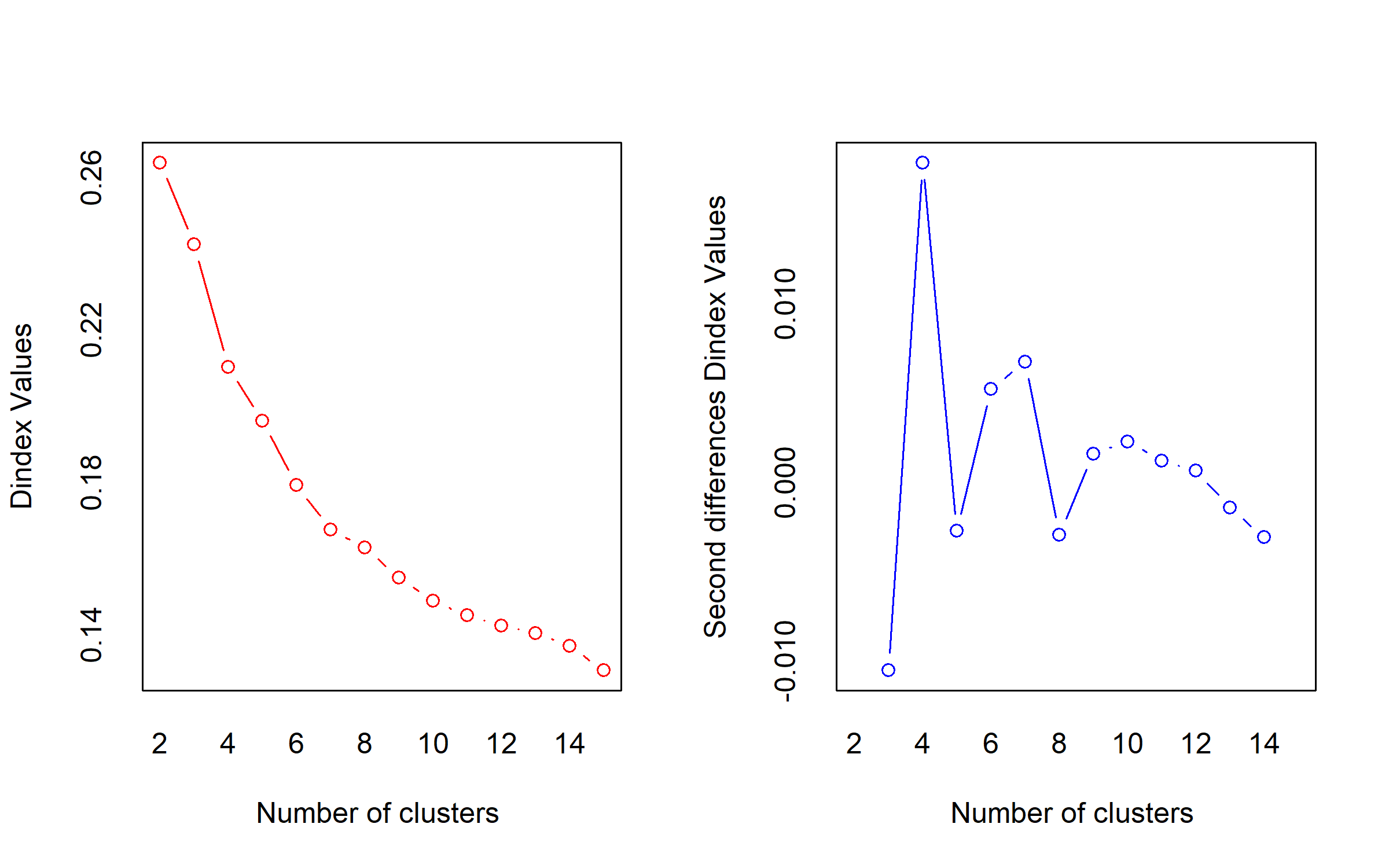
*** : The D index is a graphical method of determining the number of clusters.
                In the plot of D index, we seek a significant knee (the significant peak in Dindex
                second differences plot) that corresponds to a significant increase of the value of
                the measure.

*******************************************************************
* Among all indices:
* 4 proposed 2 as the best number of clusters
* 2 proposed 3 as the best number of clusters
* 5 proposed 4 as the best number of clusters
* 1 proposed 6 as the best number of clusters
* 2 proposed 7 as the best number of clusters
* 4 proposed 10 as the best number of clusters
* 1 proposed 13 as the best number of clusters
* 4 proposed 15 as the best number of clusters

                   ***** Conclusion *****

* According to the majority rule, the best number of clusters is  4


*******************************************************************
$All.index
KL CH Hartigan CCC Scott Marriot TrCovW TraceW
2 1.9625 72.0646 43.1709 -5.1974 236.6688 1596.8350 30.0213 19.0591
3 0.4950 63.4680 68.8217 -9.0010 353.6366 2279.2036 18.3870 16.2997
4 7.4435 76.4151 33.7409 -5.7550 633.6448 1362.9670 10.2851 12.8248
5 0.1917 73.0997 45.3120 -6.1273 761.7904 1293.4722 8.3896 11.3157
6 1.3434 77.7476 36.5987 -3.1357 944.7205 914.0985 5.8329 9.5911
7 8.0015 80.0165 15.2453 -1.1029 1053.3798 815.2061 4.7069 8.3706
8 0.1962 74.6461 25.6635 -1.6139 1100.9807 884.7331 4.0523 7.8895
9 1.0510 74.9528 23.7527 -0.5060 1206.6020 742.3897 3.5915 7.1523
10 34.9270 75.3400 12.3494 0.5180 1302.6660 630.6844 3.1240 6.5272
11 0.6694 72.1379 11.3744 0.2748 1346.8089 642.6907 2.7626 6.2163
12 0.1881 69.3630 7.7251 0.0600 1392.9727 639.0998 2.5024 5.9416
13 35.2137 65.9610 9.2750 -0.4788 1427.3519 656.1405 2.3591 5.7600
14 0.0045 63.6531 23.5850 -0.7189 1473.8089 635.1265 2.2128 5.5491
15 8.1803 66.2540 9.7789 0.7913 1589.2913 465.1975 1.8209 5.0581
Friedman Rubin Cindex DB Silhouette Duda Pseudot2 Beale Ratkowsky
2 1.1437 1.2826 0.4627 1.8797 0.2032 0.7318 46.1796 0.8779 0.1985
3 1.9536 1.4997 0.4461 1.6481 0.1752 0.6038 83.3362 1.5718 0.2320
4 4.5921 1.9061 0.4219 1.5696 0.2122 0.5819 43.8218 1.7064 0.2608
5 5.3597 2.1603 0.4035 1.3629 0.2229 0.5600 49.5005 1.8673 0.2900
6 7.3190 2.5488 0.4416 1.3070 0.2533 0.6521 35.7503 1.2692 0.2938
7 8.2513 2.9204 0.4134 1.3268 0.2640 0.6361 21.1712 1.3450 0.2906
8 8.8637 3.0985 0.4172 1.2797 0.2509 0.5048 33.3575 2.3009 0.2762
9 10.2412 3.4178 0.4039 1.1882 0.2611 0.6503 31.1912 1.2763 0.2686
10 11.4810 3.7452 0.3929 1.1489 0.2719 0.6977 21.6634 1.0255 0.2618
11 12.1036 3.9324 0.3994 1.2175 0.2483 0.7228 10.7362 0.8938 0.2523
12 12.9869 4.1143 0.4142 1.2728 0.2421 0.7429 9.3449 0.8057 0.2433
13 13.4337 4.2440 0.4148 1.2218 0.2454 0.3628 21.0719 3.9132 0.2358
14 14.1698 4.4053 0.4199 1.1575 0.2444 0.6213 22.5571 1.4331 0.2294
15 16.4827 4.8329 0.3988 1.1471 0.2608 0.5936 14.3791 1.5779 0.2256
Ball Ptbiserial Frey McClain Dunn Hubert SDindex Dindex SDbw
2 9.5296 0.3479 0.1994 0.7892 0.0697 0.0692 14.8165 0.2640 1.2413
3 5.4332 0.4039 0.1306 1.2356 0.0674 0.0793 12.2688 0.2424 0.9594
4 3.2062 0.4745 0.1319 1.9716 0.0736 0.0973 11.3109 0.2104 0.5103
5 2.2631 0.4896 0.0831 2.2104 0.0741 0.1025 10.2074 0.1962 0.4275
6 1.5985 0.5146 0.1635 2.4950 0.0878 0.1124 10.1193 0.1794 0.3865
7 1.1958 0.5217 0.1528 2.9490 0.0908 0.1237 10.1449 0.1678 0.3377
8 0.9862 0.5225 0.1245 3.0371 0.0935 0.1253 10.0881 0.1629 0.2970
9 0.7947 0.5253 0.1011 3.1675 0.0940 0.1311 10.2124 0.1551 0.3008
10 0.6527 0.5310 1.1800 3.3425 0.0974 0.1364 9.8162 0.1490 0.2538
11 0.5651 0.4957 0.2488 3.9393 0.0952 0.1407 12.9801 0.1452 0.2411
12 0.4951 0.4890 0.0694 4.1510 0.1011 0.1444 12.9797 0.1425 0.2365
13 0.4431 0.4901 0.1565 4.1792 0.1026 0.1459 13.2881 0.1406 0.2206
14 0.3964 0.4894 0.1347 4.2132 0.1045 0.1468 12.8471 0.1372 0.1994
15 0.3372 0.4845 0.1589 4.5381 0.1068 0.1548 12.7409 0.1307 0.1942
$All.CriticalValues
CritValue_Duda CritValue_PseudoT2 Fvalue_Beale
2 0.6623 64.2590 0.4769
3 0.6629 64.5683 0.1805
4 0.5863 43.0451 0.1492
5 0.5902 43.7378 0.1167
6 0.5976 45.1144 0.2824
7 0.5173 34.5247 0.2560
8 0.5041 33.4479 0.0618
9 0.5800 42.0003 0.2800
10 0.5607 39.1821 0.3952
11 0.4720 31.3281 0.4703
12 0.4656 30.9841 0.5241
13 0.3008 27.8883 0.0079
14 0.5173 34.5247 0.2259
15 0.4195 29.0549 0.1877
$Best.nc
KL CH Hartigan CCC Scott Marriot TrCovW
Number_clusters 13.0000 7.0000 4.0000 15.0000 4.0000 4.0000 3.0000
Value_Index 35.2137 80.0165 35.0808 0.7913 280.0083 846.7419 11.6342
TraceW Friedman Rubin Cindex DB Silhouette Duda
Number_clusters 4.0000 4.0000 7.0000 10.0000 15.0000 10.0000 2.0000
Value_Index 1.9658 2.6385 -0.1935 0.3929 1.1471 0.2719 0.7318
PseudoT2 Beale Ratkowsky Ball PtBiserial Frey McClain
Number_clusters 2.0000 2.0000 6.0000 3.0000 10.000 1 2.0000
Value_Index 46.1796 0.8779 0.2938 4.0964 0.531 NA 0.7892
Dunn Hubert SDindex Dindex SDbw
Number_clusters 15.0000 0 10.0000 0 15.0000
Value_Index 0.1068 0 9.8162 0 0.1942
$Best.partition
1 2 3 4 5 6 7 8 9 10 11 12 13 14 15 16 17 18 19 20
1 2 2 2 2 2 2 2 3 2 4 2 3 2 2 2 2 1 1 2
21 23 24 25 26 27 28 29 30 31 32 34 35 36 37 38 39 40 41 42
2 2 3 2 1 3 3 1 3 4 3 4 3 3 4 3 4 2 4 1
43 44 45 46 47 48 49 51 52 53 54 55 56 57 58 59 60 61 63 64
3 2 2 1 4 1 2 1 3 3 2 4 3 4 1 2 4 3 2 4
65 66 67 68 69 70 71 72 74 75 76 77 78 80 81 82 83 84 85 86
4 1 1 4 4 1 2 4 1 3 4 4 4 1 1 1 2 1 2 1
87 88 89 90 91 92 93 94 95 96 97 98 99 100 101 102 103 104 105 106
2 1 1 1 1 4 1 2 2 4 1 3 2 3 4 1 1 2 3 3
107 108 109 110 111 112 113 114 115 116 117 118 119 121 123 124 126 127 128 129
2 2 3 2 4 4 3 4 3 4 3 4 4 1 4 1 1 3 2 1
130 131 132 133 134 135 136 137 138 139 140 141 142 143 146 147 148 149 150 151
4 4 4 2 1 1 4 4 1 1 1 4 4 4 1 1 1 1 2 3
152 153 154 155 156 157 158 159 160 161 162 163 164 165 166 167 168 169 170 171
4 2 1 3 4 1 4 3 3 3 4 4 4 1 4 4 1 4 1 2
172 173 174 175 176 177 178 179 180 181 182 183 184 185 186 187 188 189 190 191
1 1 2 3 4 3 2 2 3 4 3 3 3 4 3 3 2 4 4 4
192 193 194 196 197 198 199 200 201 202 203 204 205 206 207 208 209 210 211 212
4 2 4 4 4 3 3 3 1 2 2 2 1 1 3 4 3 3 4 3
213 214 215 216 217 218 219 220 221 222 223 224 225 226 227 228 229 230 231 232
3 3 3 4 3 3 2 3 2 2 2 2 1 4 2 2 3 2 2 3
233 234 235 236 237 238 239 240 241 242 243 244 245 246 247 248 249 250 251 252
3 2 1 2 4 4 4 1 1 3 1 2 2 2 1 2 2 3 4 1
253 254 255 256 257 258 259 260 261 262 263 264 265 266 267 268 269
3 3 2 3 1 3 2 2 2 1 2 1 1 1 1 4 4 We plot the dendrogram using the suggested optimum number of clusters of 4, visualized with functions from the R package dendextend (Galili 2015). We reset the plotting window to default before that (single plot)
par(mfrow = c(1, 1))

hdend = as.dendrogram(hc_pco)
hdend = color_branches(hdend, k = 4)
hdend = color_labels(hdend, k = 4)
plot(hdend)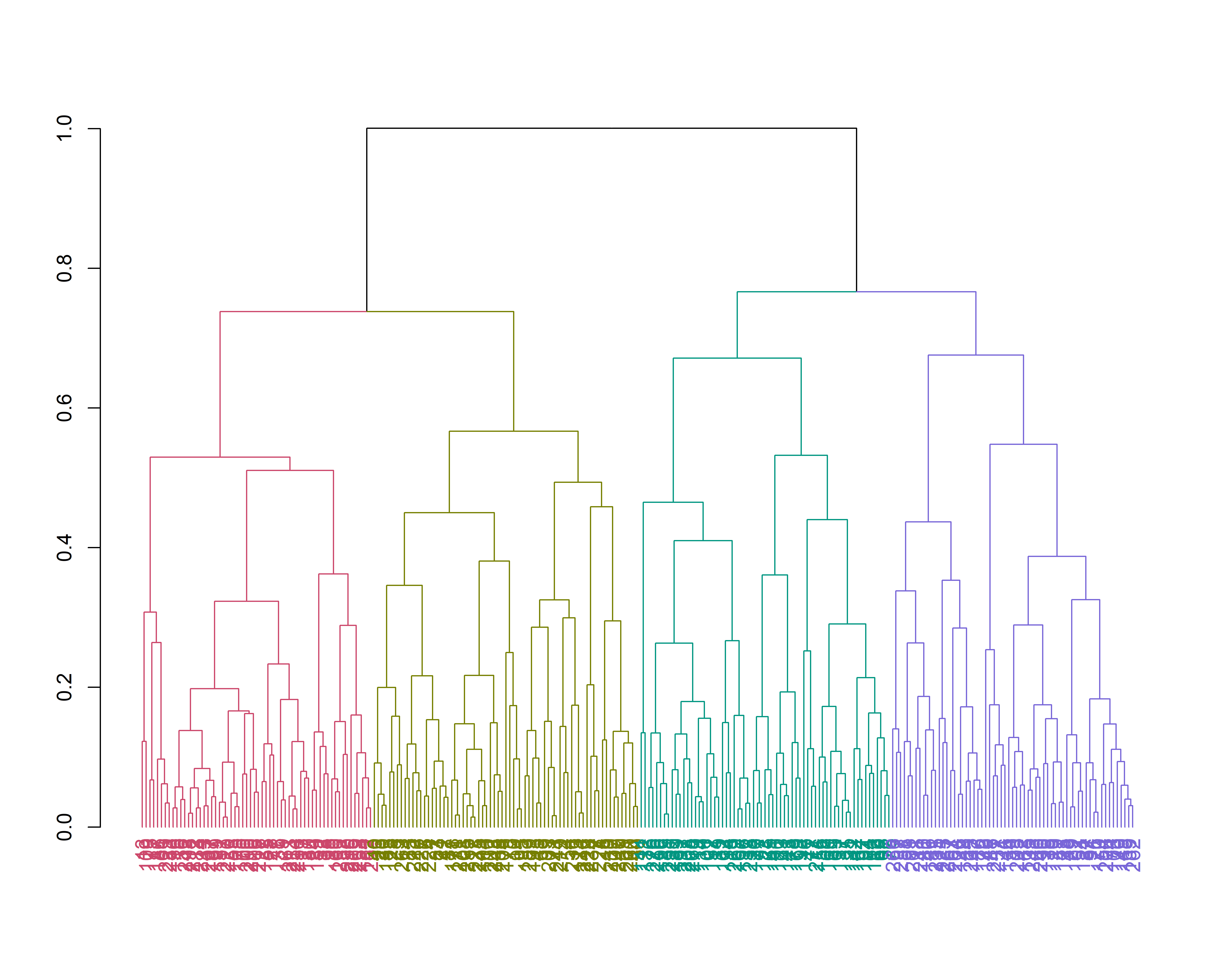
grpPCO = cutree(hc_pco, k = 4)We plot the clusters on PCO planes.
plot(pco$points[, 1], pco$points[, 2], col = grpPCO)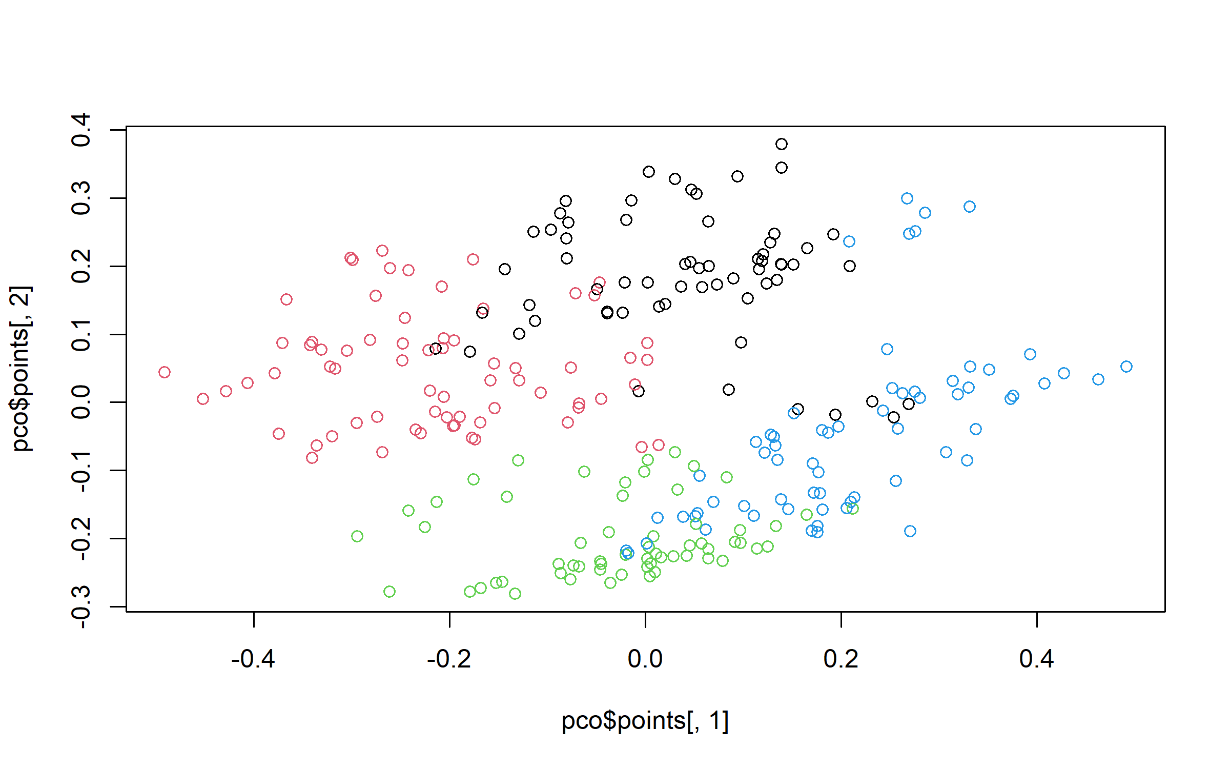
plot(pco$points[, 1], pco$points[, 3], col = grpPCO)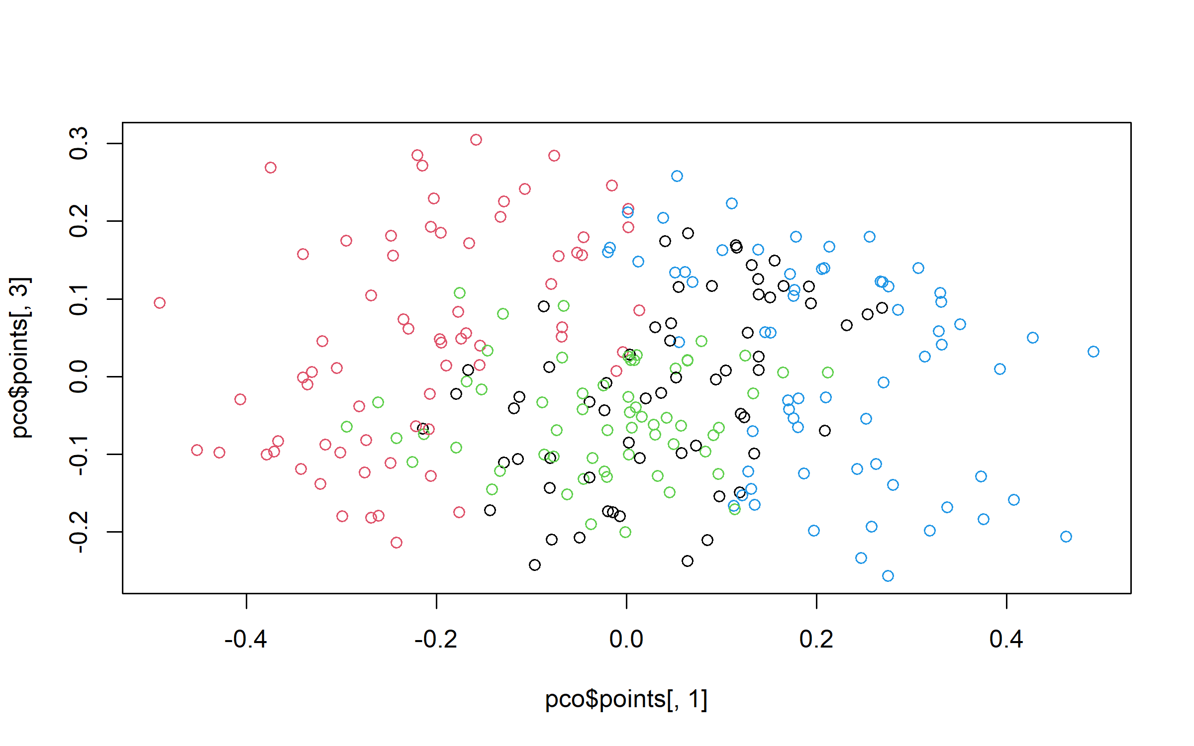
plot(pco$points[, 2], pco$points[, 3], col = grpPCO)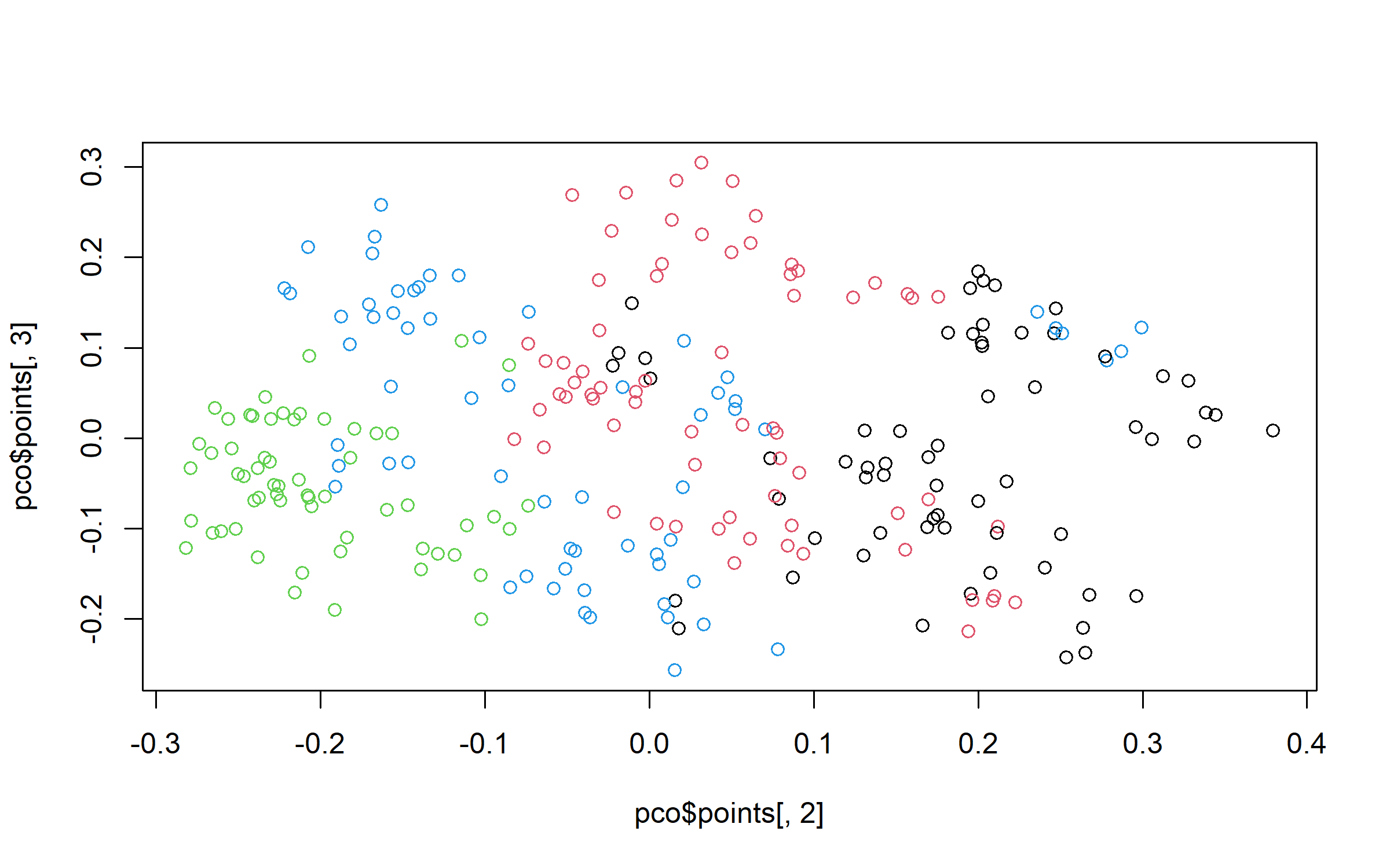
We add ‘Type’ in our dataset.
typo$type = grpPCO


data = merge(data, typo[, c(1, 41)], by = "ID")
4.4 Interpretation of the farm typology
4.4.1 Random forest
To understand which variables are the most segregating in our typology, we fit a random forest classification model and assess variable importance through the Mean Decrease in Gini index using the R package randomForest (Liaw and Wiener 2002).
In our case, the prediction is good, with a low out of bage estimate of error rate of 10.75%, and class errors for the different types between 5.19% and 18.18%.
data$type = as.factor(data$type)

rf_type = randomForest(type ~ ., data = data[, -c(1:3)], ntree = 1500)
print(rf_type)
Call:
 randomForest(formula = type ~ ., data = data[, -c(1:3)], ntree = 1500)
               Type of random forest: classification
                     Number of trees: 1500
No. of variables tried at each split: 6

        OOB estimate of  error rate: 15.95%
Confusion matrix:
   1  2  3  4 class.error
1 43 10  1  9  0.31746032
2  3 64  2  0  0.07246377
3  0  0 55  5  0.08333333
4  4  0  7 54  0.16923077
Next, we plot variable importance.
The plot shows that the most segregating variables in our typology are farming as the main source of income, and total diversity (crop and livestock).
varImpPlot(rf_type)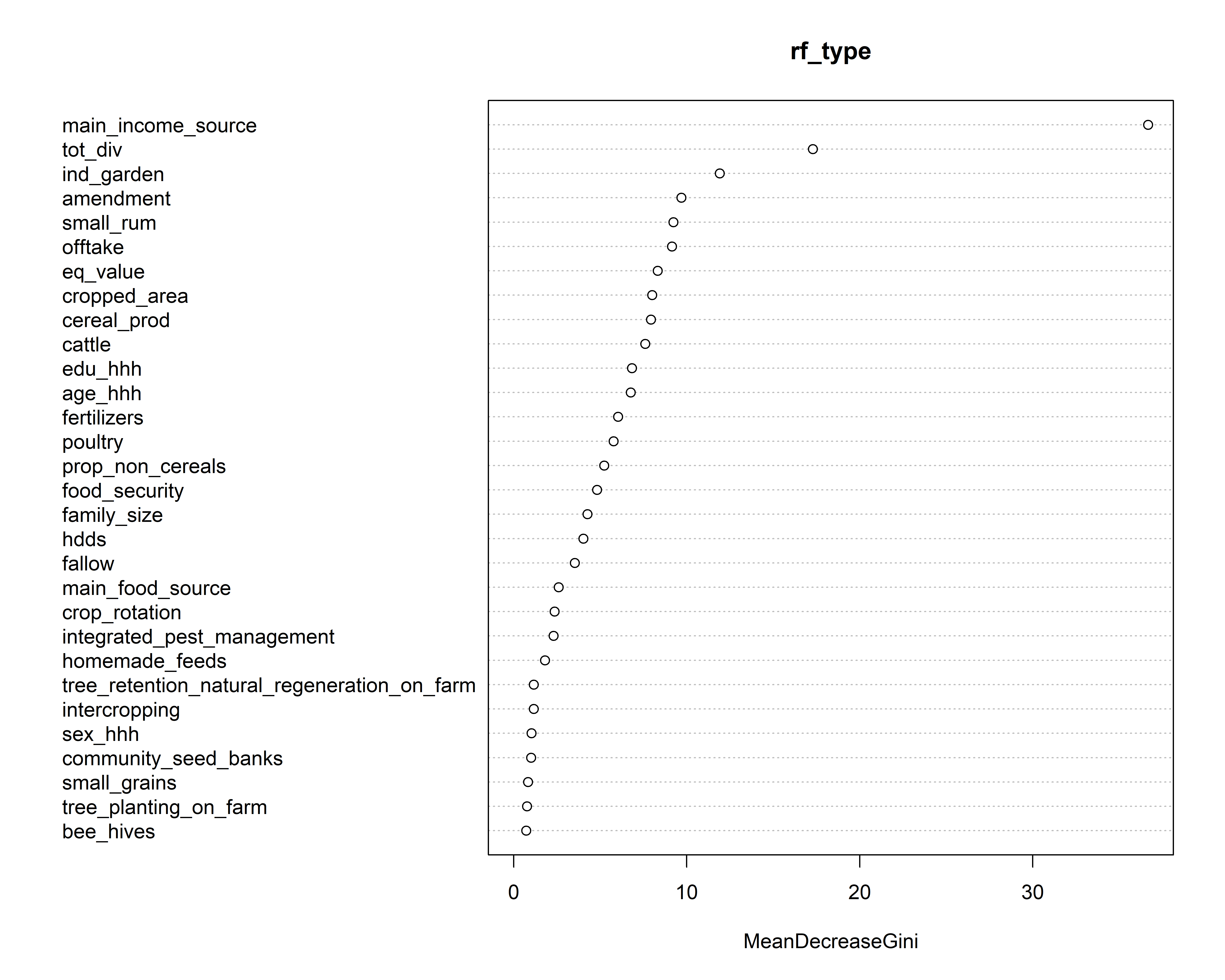
4.4.2 Summary table
To further interprete the typology, we produce a table from variables used in the delineation of the typology, displaying means and standard deviations for continuous ones and % for binary ones for the different types, using tbl_summary() from the R package gtsummary (see previous chapter.
add_p() adds a column of statistical test, and add_overall() values for the whole population.
data[, -c(1:3)] %>%
    tbl_summary(by = type, statistic = list(all_continuous() ~ "{mean} ({sd})", all_categorical() ~
        "{p}%"), type = list(hdds ~ "continuous"), digits = all_continuous() ~ 1,
        label = list(age_hhh ~ "Age of the head of the household", sex_hhh ~ "Female-headed households",
            edu_hhh ~ "Education of the head of the household higher than primary",
            family_size ~ "Family size", eq_value ~ "Equipment value (USD)", cropped_area ~
                "Total cropped area (ha)", fallow ~ "Fallow land (ha)", prop_non_cereals ~
                "Non-cereal crops (% total cropped area)", fertilizers ~ "Total fertilizer used (kg)",
            amendment ~ "Total manure + compost used (kg)", cattle ~ "Cattle (n)",
            small_rum ~ "Small ruminants (n)", poultry ~ "Poultry (n)", bee_hives ~
                "Bee keeping", ind_garden ~ "Owning an individual garden", com_garden ~
                "Having access to a communal garden", main_food_source ~ "Own production as main source of food",
            main_income_source ~ "Farming as main source of income", food_security ~
                "Proportion of the year being food secured", hdds ~ "24H household dietary diversity score (0-12)",
            community_seed_banks ~ "Using a community seed bank", small_grains ~
                "Using small grains", crop_rotation ~ "Using crop rotation", intercropping ~
                "Using intercropping", cover_crops ~ "Using cover crops", mulching ~
                "Using mulching", integrated_pest_management ~ "Using integrated pest management",
            compost_manure ~ "Using compost and manure", tree_planting_on_farm ~
                "Planting trees on-farm", tree_retention_natural_regeneration_on_farm ~
                "Retaining naturally regenerated trees on-farm", homemade_feeds ~
                "Using homemade animal feed", fodder_production ~ "Produccing fodder",
            fodder_preservation ~ "Preserving fodder", survival_feeding ~ "Using survival feeding",
            tot_div ~ "Total farm diversity (n species)", cereal_prod ~ "Total cereal production (kg/yr)",
            offtake ~ "Total livestock offtake (TLU/yr)")) %>%
    add_p(test = list(all_continuous() ~ "kruskal.test", all_categorical() ~ "chisq.test")) %>%
add_overall()| Characteristic |
Overall N = 2571 |
1 N = 631 |
2 N = 691 |
3 N = 601 |
4 N = 651 |
p-value2 |
|---|---|---|---|---|---|---|
| Age of the head of the household | 51.6 (15.8) | 50.8 (13.3) | 50.3 (16.5) | 57.0 (17.5) | 48.8 (14.7) | 0.035 |
| Female-headed households | 24% | 17% | 35% | 27% | 15% | 0.032 |
| Education of the head of the household higher than primary | 38% | 48% | 39% | 5.0% | 58% | <0.001 |
| Family size | 5.4 (2.5) | 5.9 (2.5) | 4.5 (2.1) | 4.9 (2.1) | 6.4 (3.0) | <0.001 |
| Total cropped area (ha) | 1.7 (1.4) | 1.5 (0.9) | 0.9 (0.9) | 1.9 (1.4) | 2.7 (1.7) | <0.001 |
| Fallow land (ha) | 0.7 (1.4) | 1.0 (1.1) | 0.3 (0.7) | 0.7 (1.4) | 1.0 (1.9) | <0.001 |
| Non-cereal crops (% total cropped area) | 29.3 (29.1) | 30.6 (23.6) | 15.7 (27.8) | 31.4 (32.0) | 40.5 (27.3) | <0.001 |
| Total fertilizer used (kg) | 85.6 (115.9) | 77.9 (69.3) | 32.4 (56.9) | 59.7 (72.5) | 173.7 (170.7) | <0.001 |
| Total manure + compost used (kg) | 258.0 (543.0) | 328.7 (384.9) | 29.5 (71.5) | 148.5 (454.2) | 533.2 (831.1) | <0.001 |
| Cattle (n) | 3.6 (6.7) | 2.7 (3.6) | 0.6 (2.2) | 2.0 (3.3) | 9.2 (10.4) | <0.001 |
| Small ruminants (n) | 8.5 (11.2) | 9.9 (12.1) | 2.9 (3.9) | 4.1 (4.7) | 17.0 (14.1) | <0.001 |
| Poultry (n) | 9.4 (11.3) | 10.4 (9.7) | 4.0 (5.2) | 6.8 (11.1) | 16.6 (13.5) | <0.001 |
| Bee keeping | 11% | 11% | 2.9% | 17% | 12% | 0.075 |
| Owning an individual garden | 47% | 95% | 23% | 13% | 55% | <0.001 |
| Having access to a communal garden | 1.2% | 1.6% | 0% | 1.7% | 1.5% | 0.8 |
| Own production as main source of food | 75% | 62% | 57% | 87% | 95% | <0.001 |
| Farming as main source of income | 51% | 13% | 4.3% | 100% | 91% | <0.001 |
| Proportion of the year being food secured | 0.5 (0.3) | 0.6 (0.2) | 0.4 (0.3) | 0.5 (0.3) | 0.7 (0.2) | <0.001 |
| 24H household dietary diversity score (0-12) | 3.1 (1.0) | 3.3 (0.9) | 2.8 (0.8) | 2.7 (1.0) | 3.6 (1.2) | <0.001 |
| Using a community seed bank | 12% | 6.3% | 5.8% | 23% | 12% | 0.007 |
| Using small grains | 86% | 89% | 72% | 93% | 92% | 0.001 |
| Using crop rotation | 50% | 62% | 30% | 37% | 72% | <0.001 |
| Using intercropping | 16% | 27% | 13% | 0% | 25% | <0.001 |
| Using cover crops | 8.2% | 6.3% | 5.8% | 13% | 7.7% | 0.4 |
| Using mulching | 9.7% | 13% | 1.4% | 8.3% | 17% | 0.019 |
| Using integrated pest management | 49% | 57% | 25% | 47% | 71% | <0.001 |
| Using compost and manure | 16% | 16% | 2.9% | 17% | 28% | 0.001 |
| Planting trees on-farm | 14% | 21% | 5.8% | 13% | 15% | 0.094 |
| Retaining naturally regenerated trees on-farm | 36% | 43% | 32% | 23% | 45% | 0.044 |
| Using homemade animal feed | 25% | 30% | 7.2% | 17% | 45% | <0.001 |
| Produccing fodder | 3.9% | 6.3% | 0% | 3.3% | 6.2% | 0.2 |
| Preserving fodder | 3.1% | 3.2% | 0% | 0% | 9.2% | 0.007 |
| Using survival feeding | 3.9% | 4.8% | 0% | 1.7% | 9.2% | 0.034 |
| Total farm diversity (n species) | 6.7 (3.5) | 9.1 (2.1) | 3.8 (1.8) | 4.8 (2.4) | 9.1 (3.6) | <0.001 |
| Total cereal production (kg/yr) | 839.4 (923.3) | 734.2 (790.5) | 410.5 (454.5) | 840.5 (773.1) | 1,395.8 (1,228.9) | <0.001 |
| Total livestock offtake (TLU/yr) | 0.3 (0.5) | 0.2 (0.4) | 0.1 (0.1) | 0.1 (0.3) | 0.6 (0.8) | <0.001 |
| Equipment value (USD) | 231.5 (296.5) | 207.9 (250.5) | 58.0 (91.8) | 202.5 (275.0) | 465.4 (350.4) | <0.001 |
| 1 Mean (SD); % | ||||||
| 2 Kruskal-Wallis rank sum test; Pearson’s Chi-squared test | ||||||
4.4.3 Most representative farm of each type
Finally, we pursue our interpretation of farm types by analyzing the most representative farm of each class, as the farm closest to the medoid of its farm type.
For that, we first compute distances on PCO variables.
dist_mat = dist(pco_var)We then extract medoid (e.g., the most central observation) for each cluster/farm type, and we display IDs of these medoids (row numbers from ‘data’)
medoids = sapply(unique(grpPCO), function(cl) which.min(colSums(as.matrix(dist_mat)[grpPCO ==
    cl, grpPCO == cl])))
medoids
243 17 207 156
55 13 42 38 We then retrieve the full farm data for these medoids/most representative farms.
most_representative_farms = data[medoids, ]
most_representative_farms
ID ward district age_hhh sex_hhh edu_hhh family_size cropped_area
55 363 Ward 3 9 12 17 Mbire 57 0 0 5 1.0
13 318 Ward 2 Mbire 69 0 0 8 0.5
42 349 Ward 3 9 12 17 Mbire 39 0 1 4 1.0
38 345 Ward 3 9 12 17 Mbire 60 0 0 7 0.0
fallow prop_non_cereals fertilizers amendment cattle small_rum poultry
55 2.0 0.00000 50 600 0 5 0
13 0.0 0.00000 5 0 0 0 20
42 0.8 19.98002 0 0 0 0 1
38 1.2 0.00000 10 250 0 0 0
bee_hives ind_garden com_garden main_food_source main_income_source
55 1 1 0 0 0
13 1 0 0 0 1
42 0 0 0 1 0
38 0 1 0 0 0
food_security hdds community_seed_banks small_grains crop_rotation
55 0.7500000 2 1 1 1
13 0.3333333 3 0 1 1
42 0.5000000 3 0 1 1
38 0.0000000 2 0 0 0
intercropping cover_crops mulching integrated_pest_management compost_manure
55 1 1 1 1 1
13 0 0 0 1 0
42 1 0 0 0 0
38 0 0 0 0 0
tree_planting_on_farm tree_retention_natural_regeneration_on_farm
55 1 0
13 0 0
42 0 1
38 0 0
homemade_feeds fodder_production fodder_preservation survival_feeding
55 1 1 1 0
13 0 0 0 0
42 0 0 0 0
38 0 0 0 0
tot_div cereal_prod offtake eq_value type
55 10 257 0.20 150 1
13 4 170 0.02 0 3
42 5 550 0.00 50 2
38 3 0 0.00 100 24.5 Selection of stratified samples
Typologies can be used to select a sample of farms representative of the overall population to e.g., host on-farm experiments.
Below, we select 30 representative farms using farm type as single stratum.
sample1 = as.data.frame(stratified(data, "type", 30/nrow(data)))
table(sample1$type)
1 2 3 4
7 8 7 8
We can also use more than one stratum: here we select 30 representative farms using ward (an administrative unit) and farm type as strata.
sample2 = as.data.frame(stratified(data, c("ward", "type"), 30/nrow(data)))
table(sample2$type, sample2$ward)
    Ward 2 Ward 3 9 12 17
  1      4              3
  2      5              3
  3      2              5
  4      3              4