7 Scaling
In this chapter, we assess the transferability potential of technologies generated in a specific location — the section of Mbire district where the CGIAR Agroecology Initiative was implemented. Areas sharing similar farming system, environmental, and socio-economic characteristics with the project site are assumed to have high potential for technology transfer, following the approach of Václavík et al. (2016).
We use elevation, soil texture, mean temperature, precipitation, population density, and travel time to the nearest city of at least 50,000 inhabitants as predictors. All data are downloaded via the R package geodata (Hijmans et al. 2024).
A standalone R script containing the full workflow is available at the following link: https://github.com/FBaudron/Supporting-codesign/blob/main/07-scaling/scaling.R.
7.1 Data preparation
We begin by clearing the workspace, loading the required packages, and importing the baseline dataset, which will be used to locate the project site (‘project archetype’).
rm(list = ls())

if (!require("openxlsx")) install.packages("openxlsx")
if (!require("terra")) install.packages("terra")
if (!require("geodata")) install.packages("geodata")
if (!require("ggplot2")) install.packages("ggplot2")
if (!require("ggspatial")) install.packages("ggspatial")
if (!require("tidyterra")) install.packages("tidyterra")

library(openxlsx)
library(terra)
library(geodata)
library(ggplot2)
library(ggspatial)
library(tidyterra)

data = read.xlsx("BASELINE DATA.xlsx")
7.1.1 Administrative shapefiles
We download shapefiles for Zimbabwe at country level (level 0) and province level (level 1) using the gadm() function from geodata.
zwe0 = gadm(country = "ZWE", level = 0, path = "Geodata")

plot(zwe0)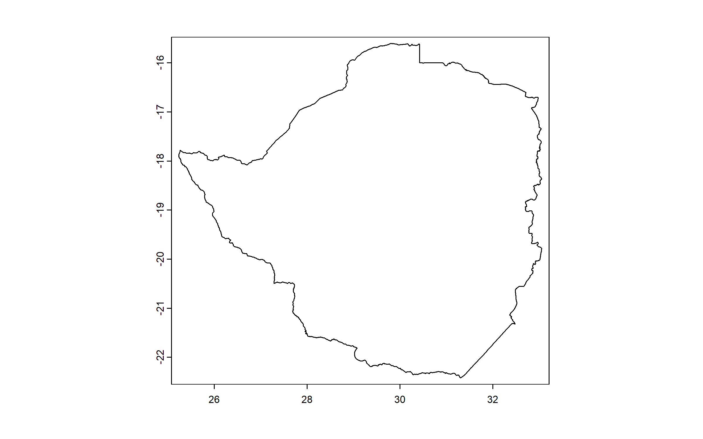
zwe1 = gadm(country = "ZWE", level = 1, path = "Geodata")

plot(zwe1)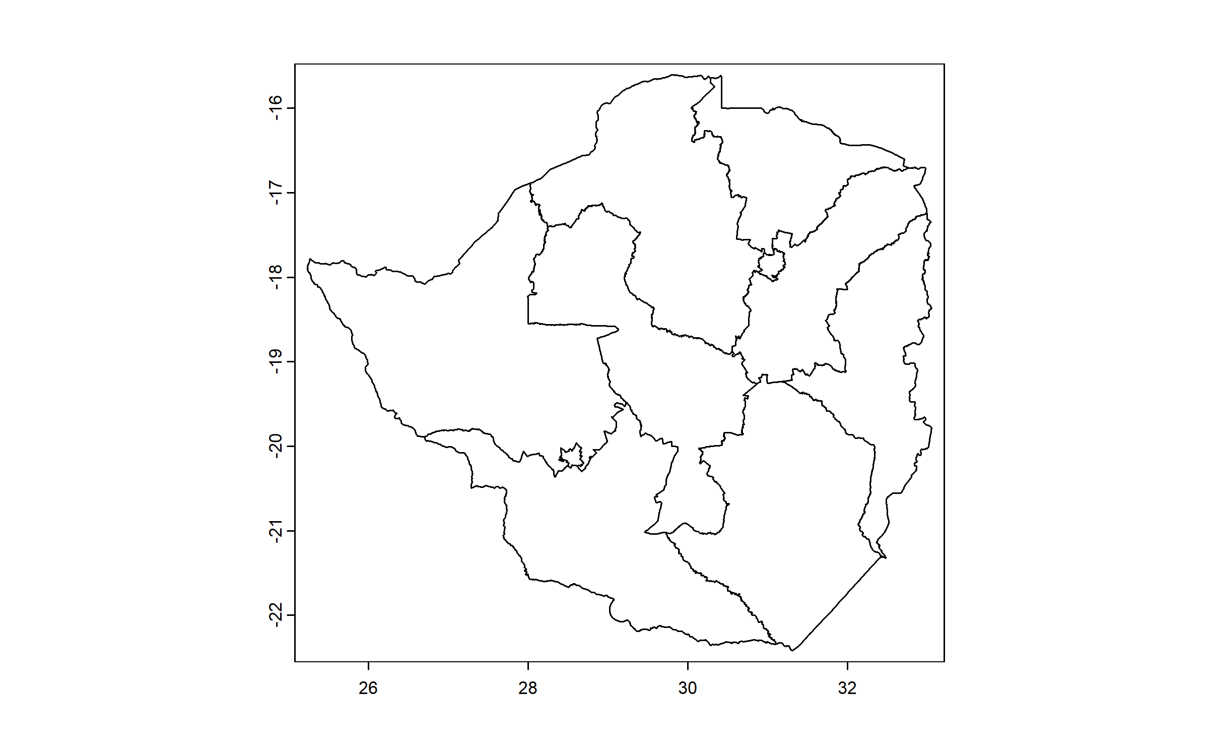
7.1.2 Cropland mask
We download a raster of probability of cropland occurrence and convert it to a presence/absence raster. We crop it to the bounding box of Zimbabwe to reduce extent (using the function crop() of terra) and mask it so that only cells within the national boundary are retained (using the function mask() of terra).
This raster represents our region of interest and will be used as a mask for all other rasters to exclude non-cropped areas.
cropland = geodata::cropland(source = "WorldCover", year = 2019, path = "Geodata")
cropland = crop(cropland, zwe0)
cropland = mask(cropland, zwe0)
cropland = ifel(cropland$cropland > 0, 1, NA)

plot(zwe0)
plot(cropland, col = "forestgreen", add = T, legend = F)
plot(zwe1, add = T)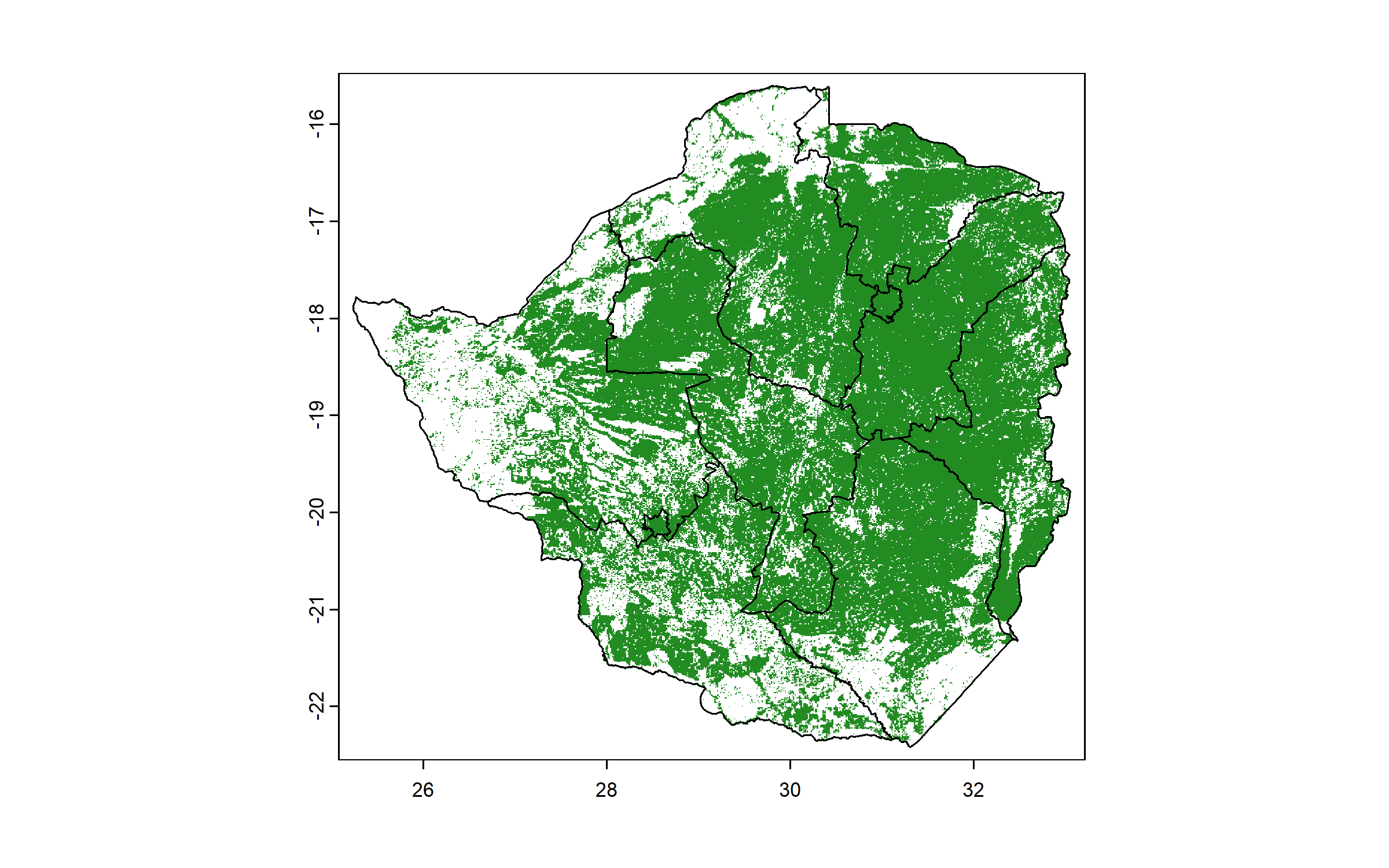
7.1.3 Rasters of predictors
We download and process rasters for all predictors, cropping and masking them to the cropland raster. We start with the raster of elevation.
elevation = geodata::elevation_30s(country = "ZWE", path = "Geodata")
elevation = crop(elevation, cropland)
elevation = mask(elevation, cropland)
names(elevation) = "elevation"

plot(zwe0)
plot(elevation, add = T, legend = T)
plot(zwe1, add = T)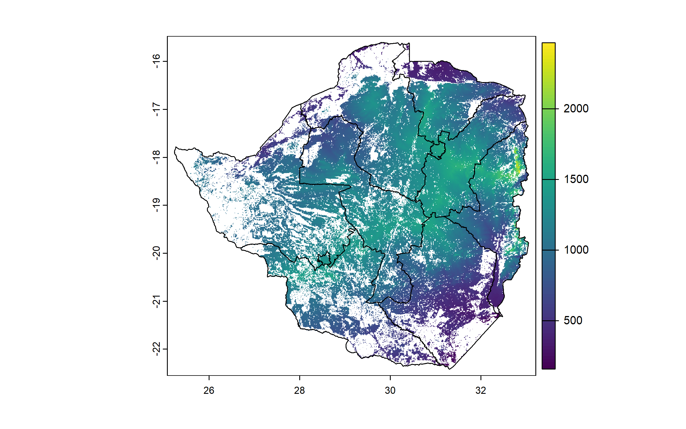
We compute a raster of weighted average of sand content across soil layers (0–5 cm, 5–15 cm, 15–30 cm), and crop and mask it to the cropland raster.
sand_5 = geodata::soil_af(var = "sand", depth = 5, path = "Geodata")
sand_15 = geodata::soil_af(var = "sand", depth = 15, path = "Geodata")
sand_30 = geodata::soil_af(var = "sand", depth = 30, path = "Geodata")
sand = (sand_5 * 5 + sand_15 * 10 + sand_30 * 15)/(5 + 10 + 15)
sand = terra::crop(sand, cropland)
sand = terra::mask(sand, cropland)
names(sand) = "sand"

plot(zwe0)
plot(sand, add = T, legend = T)
plot(zwe1, add = T)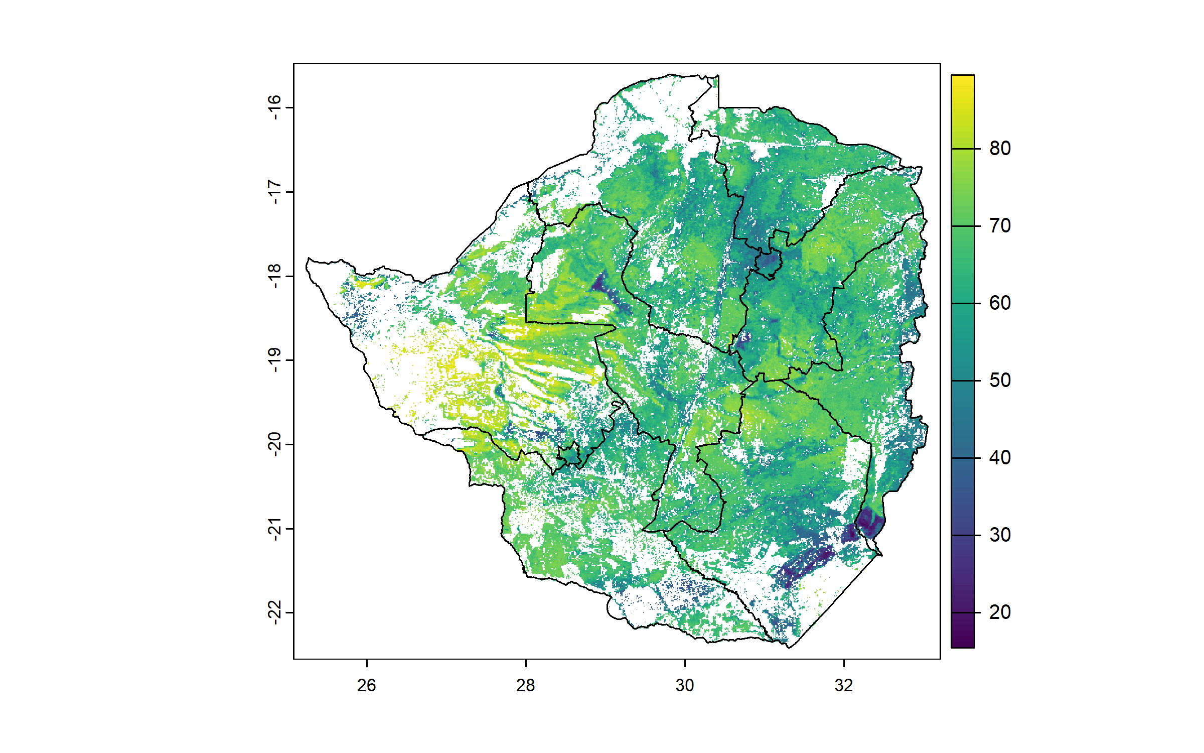
We compute a raster of mean annual temperatures, and crop and mask it to the cropland raster.
tavg = worldclim_country(country = "ZWE", var = "tavg", path = "Geodata", res = 0.5)
tavg = mean(tavg)
tavg = terra::crop(tavg, cropland)
tavg = terra::mask(tavg, cropland)
names(tavg) = "tavg"

plot(zwe0)
plot(tavg, add = T, legend = T)
plot(zwe1, add = T)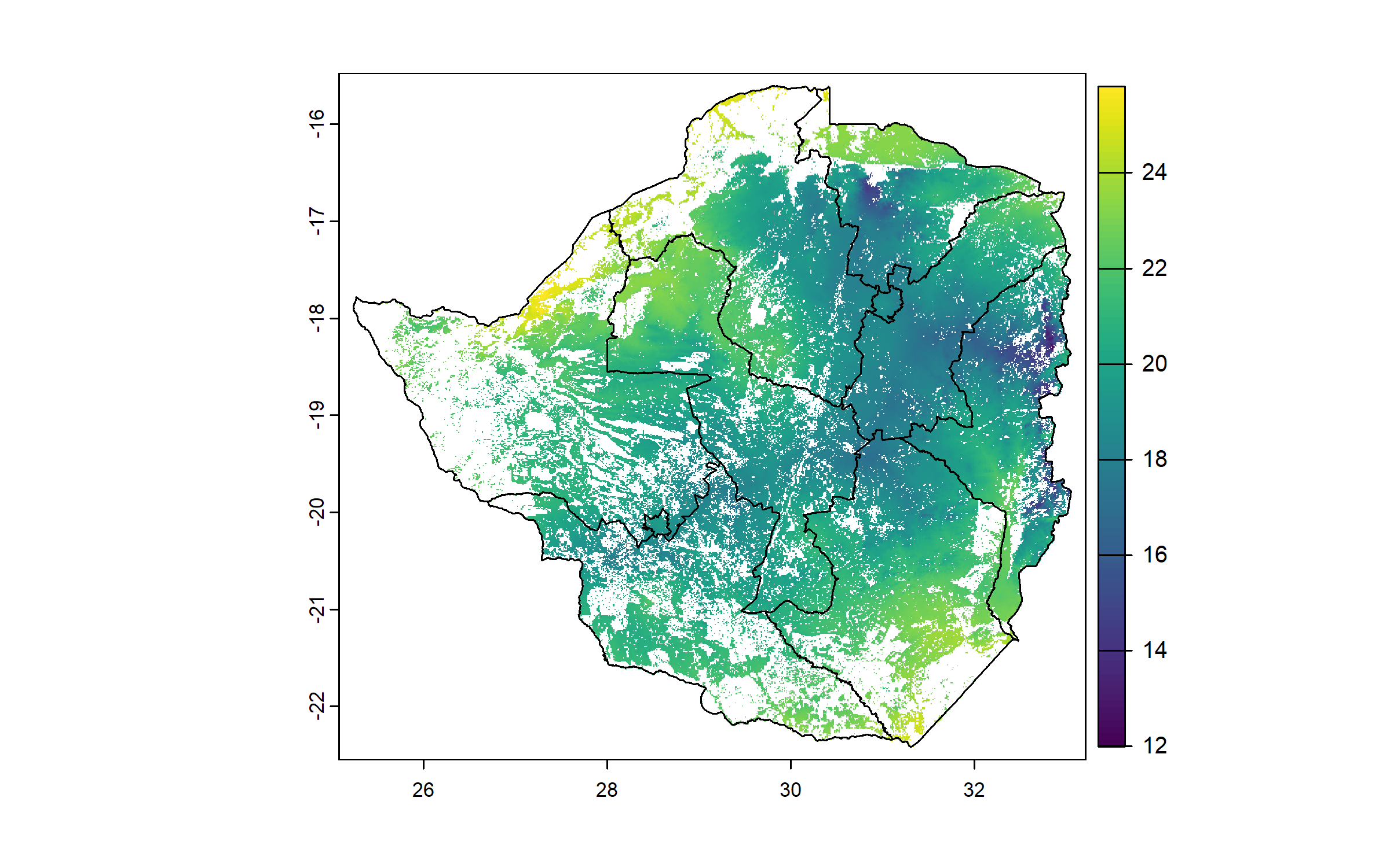
We compute a raster of annual precipitation, and crop and mask it to the cropland raster.
prec = worldclim_country(country = "ZWE", var = "prec", path = "Geodata", res = 0.5)
prec = sum(prec)
prec = terra::crop(prec, cropland)
prec = terra::mask(prec, cropland)
names(prec) = "prec"

plot(zwe0)
plot(prec, add = T, legend = T)
plot(zwe1, add = T)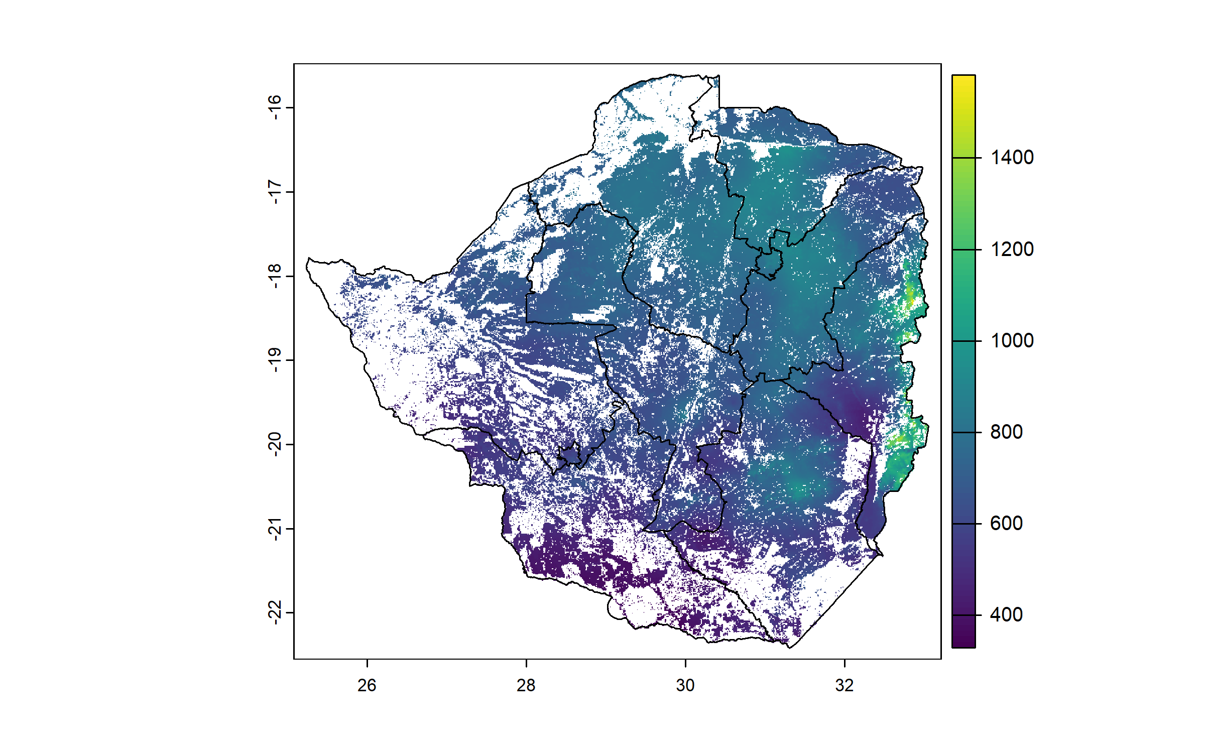
We resample the population raster to match the cropland raster resolution and extent for consistent spatial alignment, and crop and mask it to the cropland raster.
pop = geodata::population(year = 2020, path = "Geodata")
pop = resample(pop, cropland)
pop = crop(pop, cropland)
pop = mask(pop, cropland)
names(pop) = "pop"

plot(zwe0)
plot(pop, add = T, legend = T)
plot(zwe1, add = T)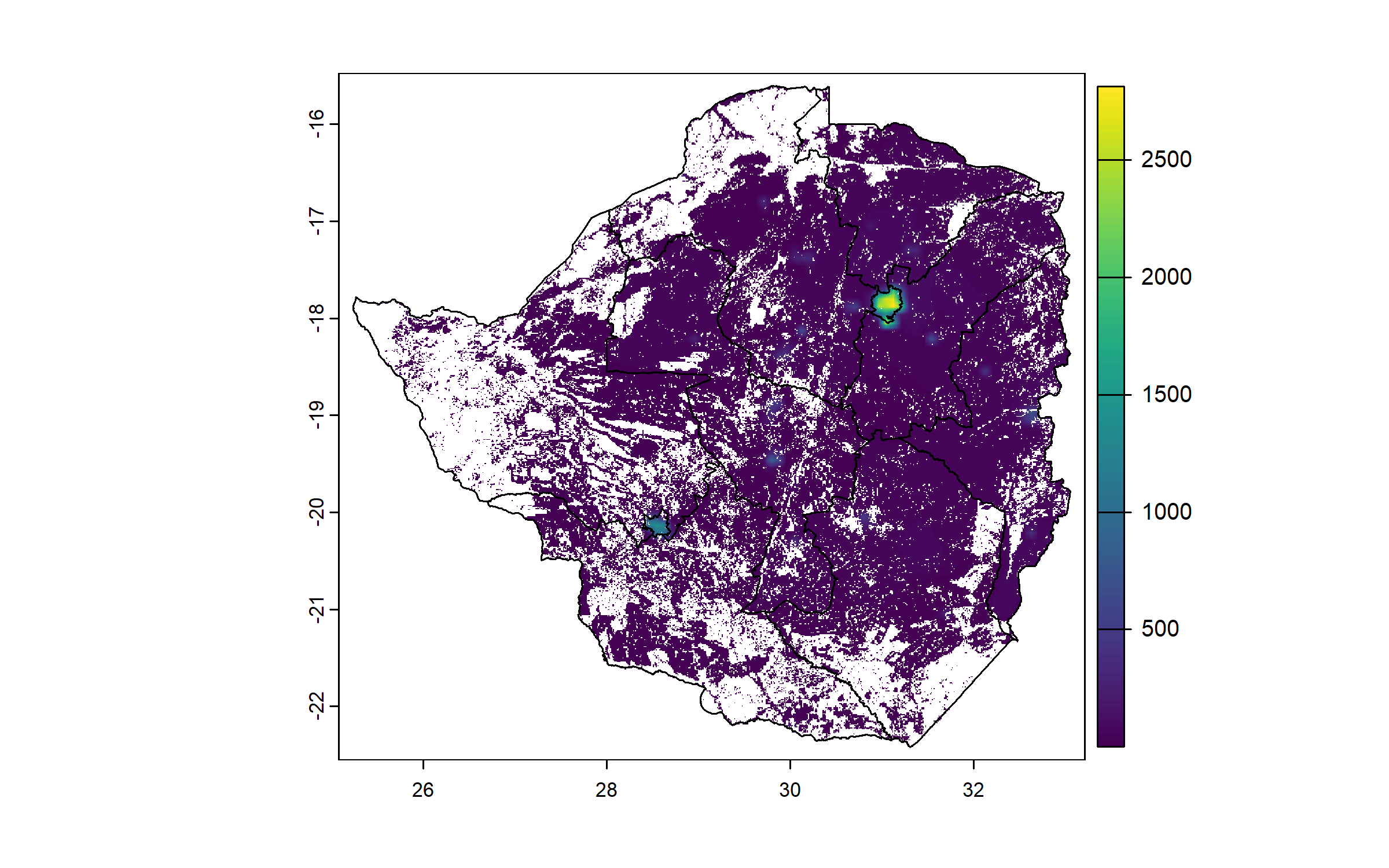
Finally, we download a raster of travel time to a city of at least 50,000 inhabitants. We crop and mask it to the cropland raster.
travel_time = travel_time(to = "city", size = 6, up = TRUE, path = "Geodata")
travel_time = crop(travel_time, cropland)
travel_time = mask(travel_time, cropland)
names(travel_time) = "travel_time"

plot(zwe0)
plot(travel_time, add = T, legend = T)
plot(zwe1, add = T)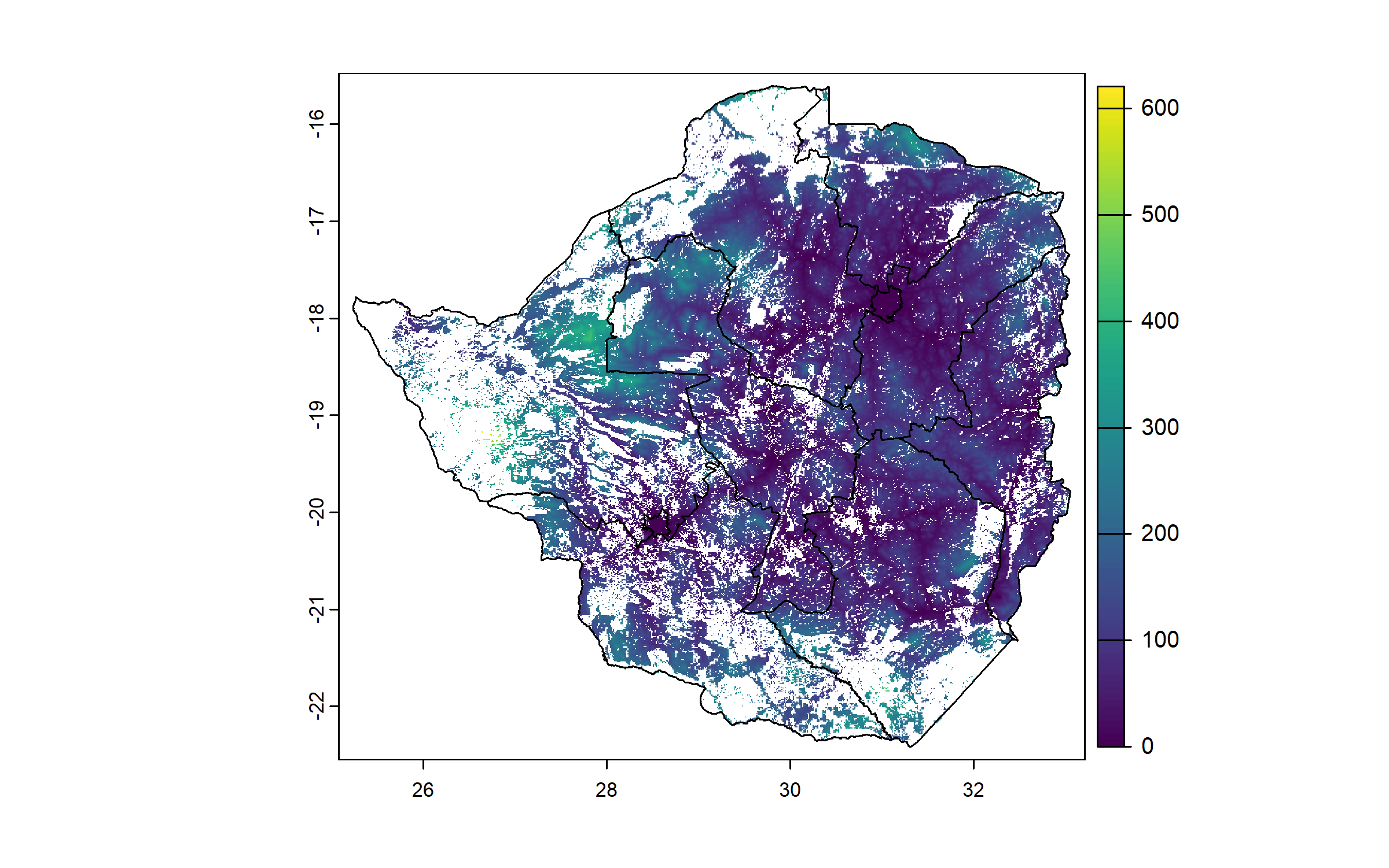
7.1.4 Preprocessing
We merge all rasters into a single stack and normalize each variable to zero mean and unit variance.
all = c(elevation, sand, tavg, prec, pop, travel_time)

means = as.numeric(global(all, "mean", na.rm = TRUE)[, 1])
sds = as.numeric(global(all, "sd", na.rm = TRUE)[, 1])
all_z = (all - means)/sds
names(all_z) = paste0(names(all), "_n")
We convert the baseline data to a spatial object, extract raster values for each surveyed farm, and compute the mean for the project site.
data_vect = vect(data, geom = c("_Record.your.current.location_longitude", "_Record.your.current.location_latitude"),
    crs = "EPSG:4326")

vals = terra::extract(all_z, data_vect)

mean_site = colMeans(vals[, -1], na.rm = TRUE)

mean_site_df = data.frame(variable = names(all_z), mean_value = mean_site)

mean_site_df
variable mean_value
elevation_n elevation_n -2.0614019
sand_n sand_n 0.3985115
tavg_n tavg_n 1.7957409
prec_n prec_n 0.2687717
pop_n pop_n -0.1931808
travel_time_n travel_time_n 0.10835647.2 Transferability potential
7.2.1 Distance to project archetype
We compute the Euclidean distance to the project archetype for each cell, following the method of Václavík et al. (2016).
We plot this raster with the centroid of the project site.
dist_to_site = sqrt(sum((all_z - mean_site)^2))

centroid = colMeans(crds(data_vect))

plot(dist_to_site, main = "Euclidean distance to project archetype")
plot(zwe1, add = T)
points(centroid["x"], centroid["y"], pch = 21, bg = "orangered", cex = 2)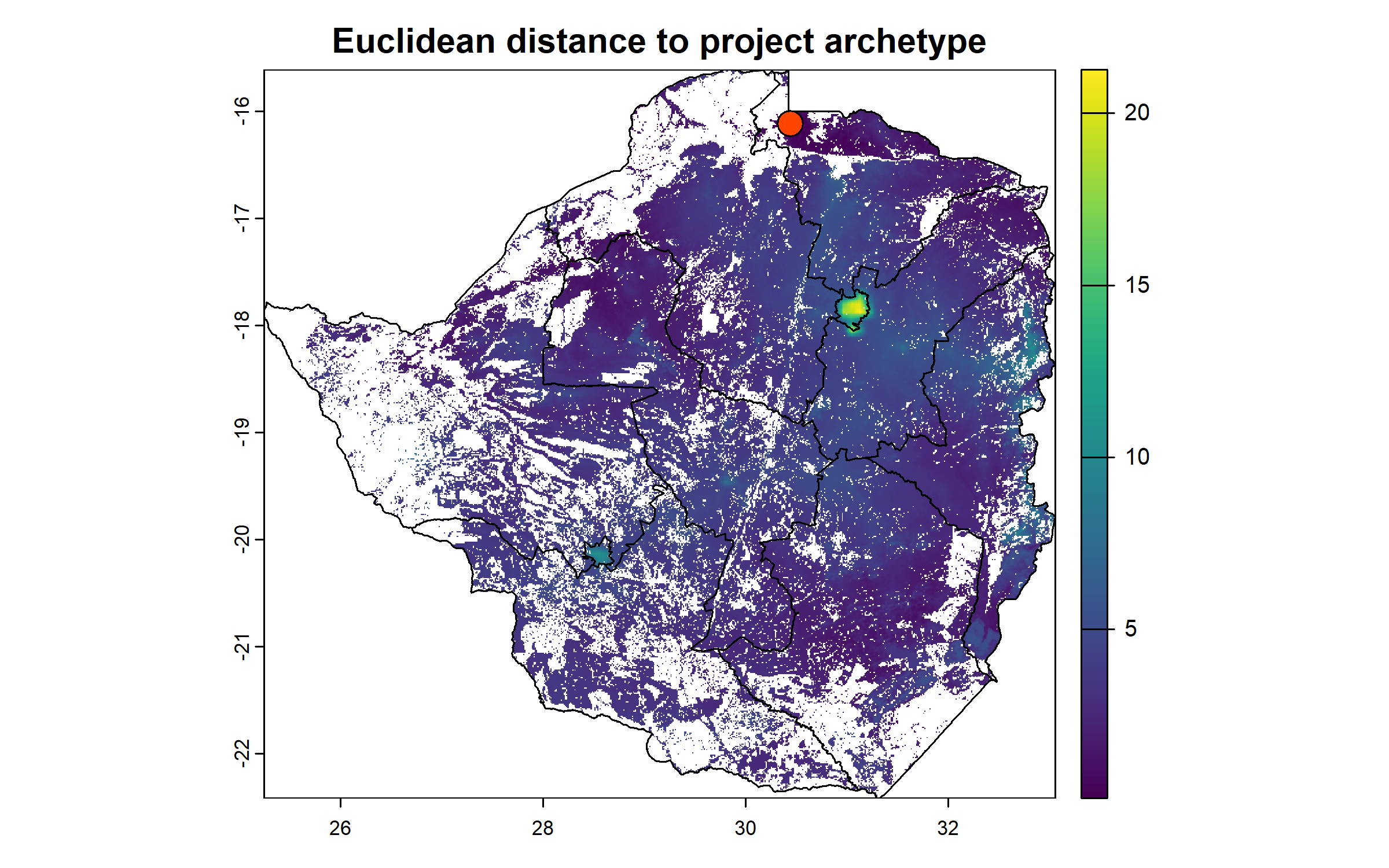
7.2.2 Transferability potential
We derive transferability potential, bounded between 0 and 1, and plot the resulting raster with the centroid of the project site.
tp_site = 1/(1 + dist_to_site)
names(tp_site) = "tp"

plot(tp_site, main = "Transferability potential")
plot(zwe1, add = T)
points(centroid["x"], centroid["y"], pch = 21, bg = "orangered", cex = 2)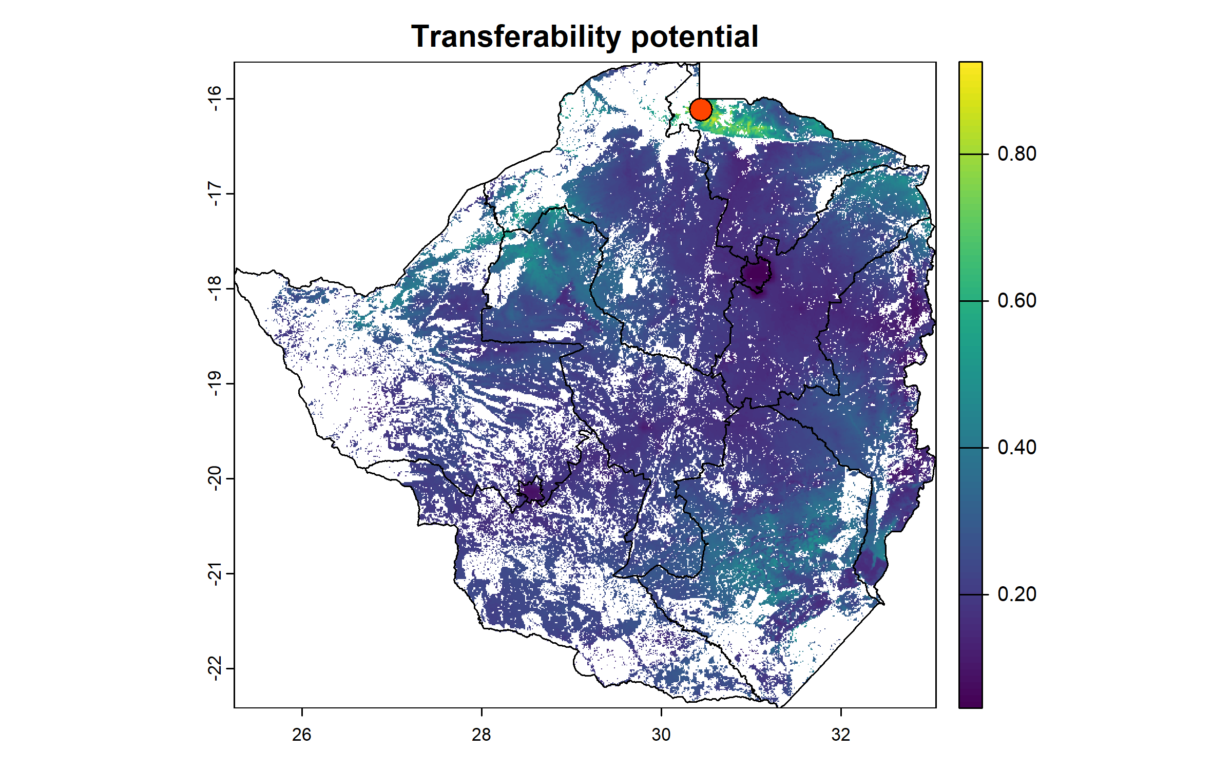
To facilitate interpretability, we discretize the raster into four classes (low, moderate, high, very high transferability) using quartiles.
tp_site_q = classify(tp_site$tp, c(quantile(values(tp_site$tp, na.rm = T))[1], quantile(values(tp_site$tp,
    na.rm = T))[2], quantile(values(tp_site$tp, na.rm = T))[3], quantile(values(tp_site$tp,
    na.rm = T))[4], quantile(values(tp_site$tp, na.rm = T))[5]))


plot(tp_site_q, type = "classes", levels = c("Low", "Moderate", "High", "Very high"),
    main = "Transferability potential")
plot(zwe1, add = T)
points(centroid["x"], centroid["y"], pch = 21, bg = "orangered", cex = 2)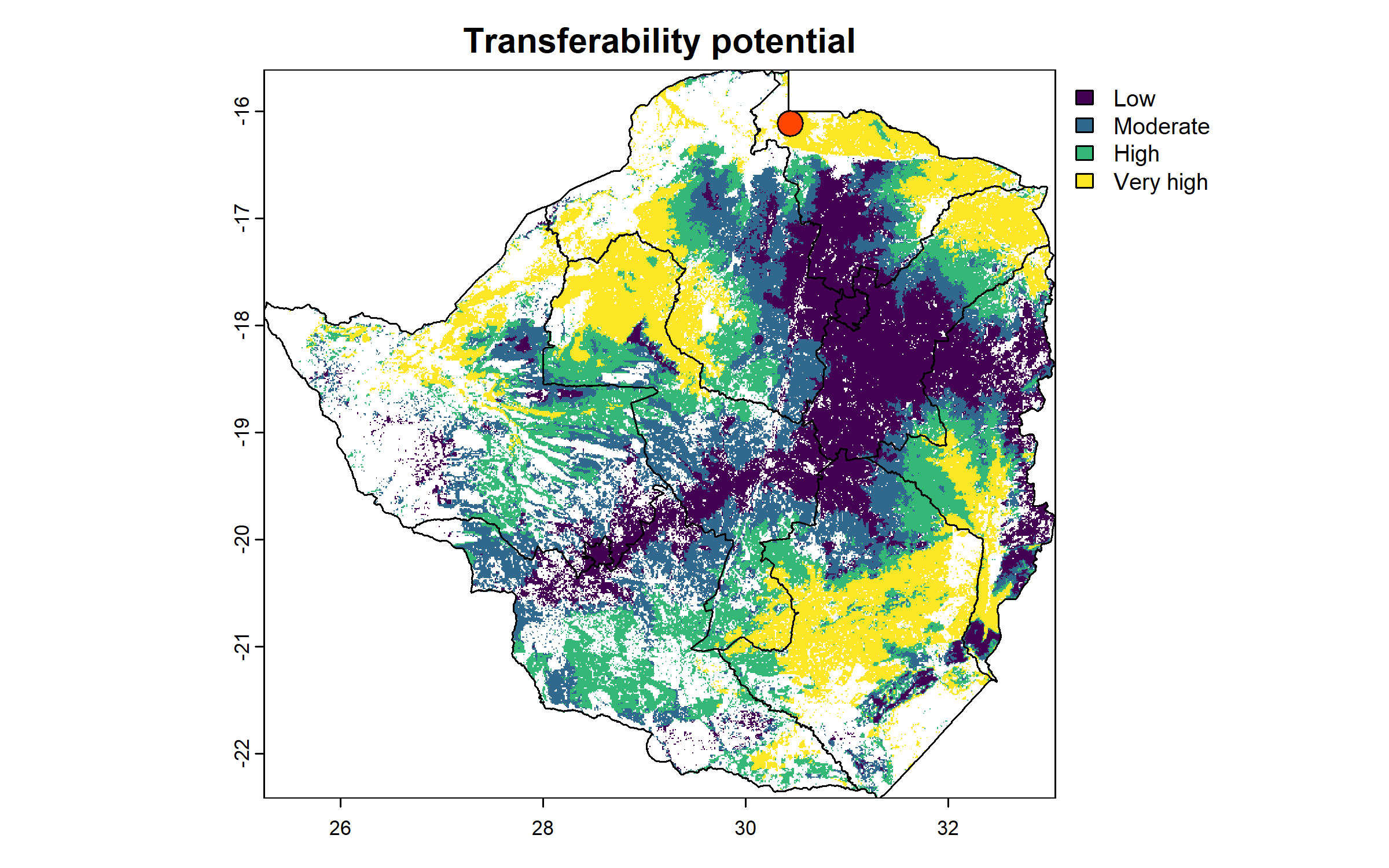
7.2.3 Publication-ready map
Below, we propose a more publication-ready version of the map using the R packages ggplot2 (Wickham 2016), tidyterra (Hernangómez 2023), and ggspatial (Dunnington 2023).
We convert the raster (and the centroid) to a dataframe, assign ordered factor labels, and plot the polished map.
tp_site_q_df = as.data.frame(tp_site_q, xy = TRUE)

names(tp_site_q_df)[3] = "class_id"

tp_site_q_df$class_id_num = as.numeric(tp_site_q_df$class_id)

tp_site_q_df$class_label = factor(tp_site_q_df$class_id_num, levels = 1:4, labels = c("Low",
    "Moderate", "High", "Very high"), ordered = TRUE)

centroid_df = data.frame(x = centroid["x"], y = centroid["y"])

ggplot() + theme_bw() + geom_raster(data = na.omit(tp_site_q_df), aes(x = x, y = y,
    fill = class_label)) + geom_spatvector(data = zwe1, fill = NA, linewidth = 1,
    color = "black") + geom_point(data = centroid_df, aes(x = x, y = y), color = "black",
    fill = "tomato", shape = 21, size = 5, stroke = 2) + scale_fill_manual(values = c(Low = "#420A68FF",
    Moderate = "#932667FF", High = "#DD513AFF", `Very high` = "#FCA50AFF")) + labs(fill = "Transferability") +
    theme(plot.title = element_blank(), axis.title = element_blank(), axis.text.y = element_text(angle = 90,
        hjust = 0.5, size = 12), axis.text.x = element_text(size = 12), legend.title = element_text(size = 14),
        legend.text = element_text(size = 12), legend.position = "right", plot.margin = ggplot2::margin(10,
            10, 10, 10)) + annotation_scale(location = "bl", width_hint = 0.5, height = unit(0.25,
    "cm"), text_cex = 1, pad_x = unit(0.15, "cm"), pad_y = unit(0.15, "cm")) + annotation_north_arrow(location = "tl",
    which_north = "true", height = unit(1, "cm"), width = unit(1, "cm"), pad_x = unit(0.15,
        "cm"), pad_y = unit(0.15, "cm"), style = north_arrow_fancy_orienteering(text_size = 10))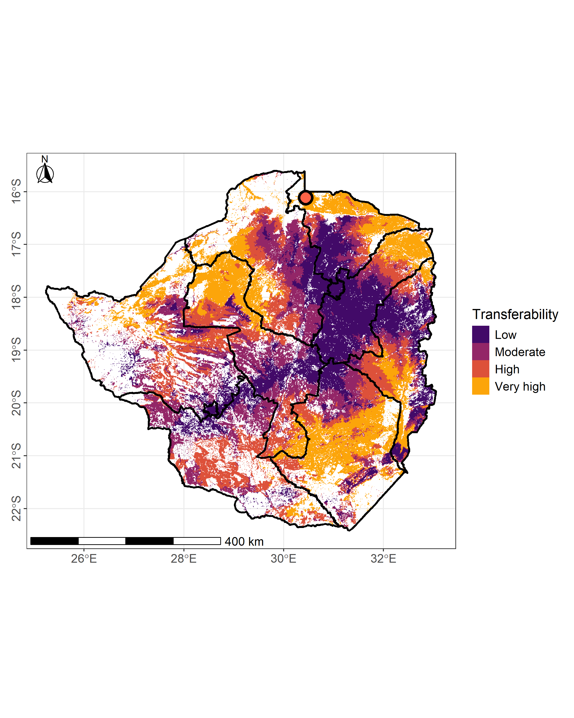
7.2.4 Area and population by transferability domain
area_tbl = zonal(cellSize(tp_site_q, unit = "km"), tp_site_q, "sum", na.rm = TRUE)
colnames(area_tbl) = c("Class", "Area_km2")

pop_tbl = zonal(pop, tp_site_q, fun = "sum", na.rm = TRUE)
colnames(pop_tbl) = c("Class", "Population")

result = merge(area_tbl, pop_tbl, by = "Class")

result$Class = c("Low", "Moderate", "High", "Very high")

result
Class Area_km2 Population
1 Low 64435.69 7306546
2 Moderate 64312.90 2525554
3 High 64213.90 2242085
4 Very high 64444.78 2435429